So you want to use force control to control the orientation of your end-effector, eh? What a noble endeavour. I, too, wished to control the orientation of the end-effector. While the journey was long and arduous, the resulting code is short and quick to implement. All of the code for reproducing the results shown here is up on my GitHub and in the ABR Control repo.
Introduction
There are numerous resources that introduce the topic of orientation control, so I’m not going to do a full rehash here. I will link to resources that I found helpful, but a quick google search will pull up many useful references on the basics.
When describing the orientation of the end-effector there are three different primary methods used: Euler angles, rotation matrices, and quaternions. The Euler angles 


Most modern robotics control is done using quaternions because they do not have singularities, and it is straight forward to convert them to other representations. Fun fact: Quaternion trajectories also interpolate nicely, where Euler angles and rotation matrices do not, so they are used in computer graphics to generate a trajectory for an object to follow in orientation space.
While you won’t need a full understanding of quaternions to use the orientation control code, it definitely helps if anything goes wrong. If you are looking to learn about or brush up on quaternions, or even if you’re not but you haven’t seen this resource, you should definitely check out these interactive videos by Grant Sanderson and Ben Eater. They have done an incredible job developing modules to give people an intuition into how quaternions work, and I can’t recommend their work enough. There’s also a non-interactive video version that covers the same material.
In control literature, angular velocity and acceleration are denoted 


How to generate task-space angular forces
So, if you recall a post long ago on Jacobians, our task-space Jacobian has 6 rows:
![\left[ \begin{array}{c} \dot{\textbf{x}} \\ \pmb{\omega} \end{array} \right] = \textbf{J}(\textbf{q}) \; \dot{\textbf{q}}](https://s0.wp.com/latex.php?latex=%5Cleft%5B+%5Cbegin%7Barray%7D%7Bc%7D+%5Cdot%7B%5Ctextbf%7Bx%7D%7D+%5C%5C+%5Cpmb%7B%5Comega%7D+%5Cend%7Barray%7D+%5Cright%5D+%3D+%5Ctextbf%7BJ%7D%28%5Ctextbf%7Bq%7D%29+%5C%3B+%5Cdot%7B%5Ctextbf%7Bq%7D%7D&bg=ffffff&fg=555555&s=0&c=20201002)
In position control, where we’re only concerned about the 
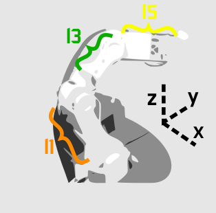
Now that we’re interested in orientation control, however, we will need to learn up (and thank you to Yitao Ding for clarifying this point in comments on the original version of this post). The Jacobian for the orientation describes the rotational velocities around each axis
To generate our task-space angular forces we will have to generate an orientation angle error signal of the appropriate form. To do that, first we’re going to have to get and be able to manipulate the orientation representation of the end-effector and our target.
Transforming orientation between representations
We can get the current end-effector orientation in rotation matrix form quickly, using the transformation matrices for the robot. To get the target end-effector orientation in the examples below we’ll use the VREP remote API, which returns Euler angles.
It’s important to note that Euler angles can come in 12 different formats. You have to know what kind of Euler angles you’re dealing with (e.g. rotate around X then Y then Z, or rotate around X then Y then X, etc) for all of this to work properly. It should be well documented somewhere, for example the VREP API page tells us that it will return angles corresponding to x, y, and then z rotations.
The axes of rotation can be static (extrinsic rotations) or rotating (intrinsic rotations). NOTE: The VREP page says that they rotate around an absolute frame of reference, which I take to mean static, but I believe that’s a typo on their page. If you calculate the orientation of the end-effector of the UR5 using transform matrices, and then convert it to Euler angles with axes='rxyz' you get a match with the displayed Euler angles, but not with axes='sxyz'.
Now we’re going to have to be able to transform between Euler angles, rotation matrices, and quaternions. There are well established methods for doing this, and a bunch of people have coded things up to do it efficiently. Here I use the very handy transformations module from Christoph Gohlke at the University of California. Importantly, when converting to quaternions, don’t forget to normalize the quaternions to unit length.
from abr_control.arms import ur5 as arm
from abr_control.interfaces import VREP
from abr_control.utils import transformations

robot_config = arm.Config()
interface = VREP(robot_config)
interface.connect()

feedback = interface.get_feedback()
# get the end-effector orientation matrix
R_e = robot_config.R('EE', q=feedback['q'])
# calculate the end-effector unit quaternion
q_e = transformations.unit_vector(
    transformations.quaternion_from_matrix(R_e))

# get the target information from VREP
target = np.hstack([
    interface.get_xyz('target'),
    interface.get_orientation('target')])
# calculate the target orientation rotation matrix
R_d = transformations.euler_matrix(
    target[3], target[4], target[5], axes='rxyz')[:3, :3]
# calculate the target orientation unit quaternion
q_d = transformations.unit_vector(
    transformations.quaternion_from_euler(
        target[3], target[4], target[5],
        axes='rxyz'))  # converting angles from 'rotating xyz'
Generating the orientation error
I implemented 4 different methods for calculating the orientation error, from (Caccavale et al, 1998), (Yuan, 1988) and (Nakinishi et al, 2008), and then one based off some code I found on Stack Overflow. I’ll describe each below, and then we’ll look at the results of applying them in VREP.
Method 1 – Based on code from StackOverflow
Given two orientation quaternion 


To isolate 


Great! Now we know how to calculate the rotation needed to get from the current orientation to the target orientation. Next, we have to get from
For control purposes, the last three elements of the quaternion define the roll, pitch, and yaw rotational errors…
So you can just take the vector part of the quaternion
# calculate the rotation between current and target orientations
q_r = transformations.quaternion_multiply(
    q_target, transformations.quaternion_conjugate(q_e))

# convert rotation quaternion to Euler angle forces
u_task[3:] = ko * q_r[1:] * np.sign(q_r[0])
NOTE: You will run into issues when the angle 
q_r[1:] * np.sign(q_r[0]). This will make sure that you always rotate along a trajectory < 180 degrees towards the target angle. The reason that this crops up is because there are multiple different quaternions that can represent the same orientation.
The following figure shows the arm being directed from and to the same orientations, where the one on the left takes the long way around, and the one on the right multiplies by the sign of the scalar component of the
Method 2 – Quaternion feedback from Resolved-acceleration control of robot manipulators: A critical review with experiments (Caccavale et al, 1998)
In section IV, equation (34) of this paper they specify the orientation error to be calculated as

where 


To implement this is pretty straight forward using the transforms.py module to handle the representation conversions:
# From (Caccavale et al, 1997)
# Section IV - Quaternion feedback
R_ed = np.dot(R_e.T, R_d)  # eq 24
q_ed = transformations.quaternion_from_matrix(R_ed)
q_ed = transformations.unit_vector(q_ed)
u_task[3:] = -np.dot(R_e, q_ed[1:])  # eq 34
Method 3 – Angle/axis feedback from Resolved-acceleration control of robot manipulators: A critical review with experiments (Caccavale et al, 1998)
In section V of the paper, they present an angle / axis feedback algorithm, which overcomes the singularity issues that classic Euler angle methods suffer from. The algorithm defines the orientation error in equation (45) to be calculated
where 


Where 
# From (Caccavale et al, 1997)
# Section V - Angle/axis feedback
R_de = np.dot(R_d, R_e.T)  # eq 44
q_ed = transformations.quaternion_from_matrix(R_de)
q_ed = transformations.unit_vector(q_ed)
u_task[3:] = -2 * q_ed[0] * q_ed[1:]  # eq 45
From playing around with this briefly, it seems like this method also works. The authors note in the discussion that it may “suffer in the case of large orientation errors”, but I wasn’t able to elicit poor behaviour when playing around with it in VREP. The other downside they mention is that the computational burden is heavier with this method than with quaternion feedback.
Method 4 – From Closed-loop manipulater control using quaternion feedback (Yuan, 1988) and Operational space control: A theoretical and empirical comparison (Nakanishi et al, 2008)
This was the one method that I wasn’t able to get implemented / working properly. Originally presented in (Yuan, 1988), and then modified for representing the angular velocity in world and not local coordinates in (Nakanishi et al, 2008), the equation for generating error (Nakanishi eq 72):

where 


![\left[ \begin{array}{ccc} 0 & -\textbf{x}[2] & \textbf{x}[1] \\ \textbf{x}[2] & 0 & -\textbf{x}[0] \\ -\textbf{x}[1] & \textbf{x}[0] & 0 \end{array} \right]](https://s0.wp.com/latex.php?latex=%5Cleft%5B+%5Cbegin%7Barray%7D%7Bccc%7D+0+%26+-%5Ctextbf%7Bx%7D%5B2%5D+%26+%5Ctextbf%7Bx%7D%5B1%5D+%5C%5C+%5Ctextbf%7Bx%7D%5B2%5D+%26+0+%26+-%5Ctextbf%7Bx%7D%5B0%5D+%5C%5C+-%5Ctextbf%7Bx%7D%5B1%5D+%26+%5Ctextbf%7Bx%7D%5B0%5D+%26+0+%5Cend%7Barray%7D+%5Cright%5D&bg=ffffff&fg=555555&s=0&c=20201002)
My code for this implementation looks like:
S = np.array([
    [0.0, -q_d[2], q_d[1]],
    [q_d[2], 0.0, -q_d[0]],
    [-q_d[1], q_d[0], 0.0]])

u_task[3:] = -(q_d[0] * q_e[1:] - q_e[0] * q_d[1:] +
               np.dot(S, q_e[1:]))
If you understand why this isn’t working, if you can provide a working code example in the comments I would be very grateful.
Generating the full orientation control signal
The above steps generate the task-space control signal, and from here I’m just using standard operational space control methods to take u_task and transform it into joint torques to send out to the arm. With possibly the caveat that I’m accounting for velocity in joint-space, not task space. Generating the full control signal looks like:
# which dim to control of [x, y, z, alpha, beta, gamma]
ctrlr_dof = np.array([False, False, False, True, True, True])

feedback = interface.get_feedback()
# get the end-effector orientation matrix
R_e = robot_config.R('EE', q=feedback['q'])
# calculate the end-effector unit quaternion
q_e = transformations.unit_vector(
    transformations.quaternion_from_matrix(R_e))

# get the target information from VREP
target = np.hstack([
    interface.get_xyz('target'),
    interface.get_orientation('target')])
# calculate the target orientation rotation matrix
R_d = transformations.euler_matrix(
    target[3], target[4], target[5], axes='rxyz')[:3, :3]
# calculate the target orientation unit quaternion
q_d = transformations.unit_vector(
    transformations.quaternion_from_euler(
        target[3], target[4], target[5],
        axes='rxyz'))  # converting angles from 'rotating xyz'

# calculate the Jacobian for the end effectora
# and isolate relevate dimensions
J = robot_config.J('EE', q=feedback['q'])[ctrlr_dof]

# calculate the inertia matrix in task space
M = robot_config.M(q=feedback['q'])

# calculate the inertia matrix in task space
M_inv = np.linalg.inv(M)
Mx_inv = np.dot(J, np.dot(M_inv, J.T))
if np.linalg.det(Mx_inv) != 0:
    # do the linalg inverse if matrix is non-singular
    # because it's faster and more accurate
    Mx = np.linalg.inv(Mx_inv)
else:
    # using the rcond to set singular values < thresh to 0
    # singular values < (rcond * max(singular_values)) set to 0
    Mx = np.linalg.pinv(Mx_inv, rcond=.005)

u_task = np.zeros(6)  # [x, y, z, alpha, beta, gamma]

# generate orientation error
# CODE FROM ONE OF ABOVE METHODS HERE

# remove uncontrolled dimensions from u_task
u_task = u_task[ctrlr_dof]

# transform from operational space to torques and
# add in velocity and gravity compensation in joint space
u = (np.dot(J.T, np.dot(Mx, u_task)) -
     kv * np.dot(M, feedback['dq']) -
     robot_config.g(q=feedback['q']))

# apply the control signal, step the sim forward
interface.send_forces(u)
The control script in full context is available up on my GitHub along with the corresponding VREP scene. If you download and run both (and have the ABR Control repo installed), then you can generate fun videos like the following:
Method 1 – Stack overflow code 
Method 2 – Caccavale quaternion
Method 3 – Caccavale angle/axis 
Method 4 – Yuan / Nakanishi
Here, the green ball is the target, and the end-effector is being controlled to match the orientation of the ball. The blue box is just a visualization aid for displaying the orientation of the end-effector. And that hand is on there just from another project I was working on then forgot to remove but already made the videos so here we are. It’s set to not affect the dynamics so don’t worry. The target changes orientation once a second. The orientation gain for these trials is ko=200 and kv=np.sqrt(600).
The first three methods all perform relatively similarly to each other, although method 3 seems to be a bit faster to converge to the target orientation after the first movement. But it’s pretty clear something is terribly wrong with the implementation of the Yuan algorithm in method 4; brownie points for whoever figures out what!
Controlling position and orientation
So you want to use force control to control both position and orientation, eh? You are truly reaching for the stars, and I applaud you. For the most part, this is pretty straight-forward. But there are a couple of gotchyas so I’ll explicitly go through the process here.
How many degrees-of-freedom (DOF) can be controlled?
If you recall from my article on Jacobians, there was a section on analysing the Jacobian. It comes down to two main points: 1) The Jacobian specifies which task-space DOF can be controlled. If there is a row of zeros, for example, the corresponding task-space DOF (i.e. 
For example, in a two joint planar arm, the 


controlling 3 DOF 
controlling 2 DOF
How to specify which DOF are being controlled?
Okay, so we don’t want to try to control too many DOF at once. Got it. Let’s say we know that our arm has 3 DOF, how do we choose which DOF to control? Simple: You remove the rows from you Jacobian and your control signal that correspond to task-space DOF you don’t want to control.
To implement this in code in a flexible way, I’ve chosen to specify an array with 6 boolean elements, set to True if you want to control the corresponding task space parameter and False if you don’t. For example, if you to control just the ctrl_dof = [True, True, True, False, False, False].
We then strip the Jacobian and task space control signal down to the relevant rows with J = robot_config.('EE', q)[ctrlr_dof] and u_task = (current - target)[ctrlr_dof]. This means that both current and target must be 6-dimensional vectors specifying the current and target
Generating a position + orientation control signal
The UR5 has 6 degrees of freedom, so we’re able to fully control the task space position and orientation. To do this, in the above script just ctrl_dof = np.array([True, True, True, True, True, True]), and there you go! In the following animations the gain values used were kp=300, ko=300, and kv=np.sqrt(kp+ko)*1.5. The full script can be found up on my GitHub.
Method 1 – Stack overflow code 
Method 2 – Caccavale quaternion
Method 3 – Caccavale angle/axis 
Method 4 – Yuan / Nakanishi
NOTE: Setting the gains properly for this task is pretty critical, and I did it just by trial and error until I got something that was decent for each. For a real comparison, better parameter tuning would have to be undertaken more rigorously.
NOTE: When implementing this minimal code example script I ran into a problem that was caused by the task-space inertia matrix calculation. It turns out that using np.linalg.pinv gives very different results than np.linalg.inv, and I did not realise this. I’m going to have to explore this more fully later, but basically heads up that you want to be using np.linalg.inv as much as possible. So you’ll notice in the above code I check the dimensionality of Mx_inv and first try to use np.linalg.inv before resorting to np.linalg.pinv.
NOTE: If you start playing around with controlling only one or two of the orientation angles, something to keep in mind: Because we’re using rotating axes, if you set up False, False, True then it’s not going to look like
In summary
So that’s that! Lots of caveats, notes, and more work to be done, but hopefully this will be a useful resource for any others embarking on the same journey. You can download the code, try it out, and play around with the gains and targets. Let me know below if you have any questions or enjoyed the post, or want to share any other resources on force control of task-space orientation.
And once again thanks to Yitao Ding for his helpful comments and corrections on the original version of this article.
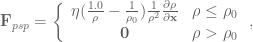
 is the distance to the target,
  is the threshold distance to the target at which point the avoidance function activates,
  is the partial derivative of the distance to the target with respect to a given point on the arm, and
  is a gain term.
 , and gets huge as the obstacle nears the object (as
  ). Using
  and
and  gives us a function that looks like
 locations of arm segment (which we are assuming is a straight line), and


 using the equation we defined above. The one part of that equation that wasn’t specified was exactly what
 is the Jacobian for the point of interest,
  is the operational space inertia matrix for the point of interest, and
  is the force we defined above.
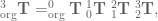
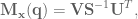
 reads the transform from reference frame
  to reference frame
  .
. , we multiply it by the point of interest in reference frame 3, which, previously, has usually been
 ![\textbf{x} = [0, 0, 0]](https://s0.wp.com/latex.php?latex=%5Ctextbf%7Bx%7D+%3D+%5B0%2C+0%2C+0%5D&bg=ffffff&fg=555555&s=0&c=20201002) . In other words, usually we’re just interested in the origin of reference frame 3. So the Jacobian is just
. In other words, usually we’re just interested in the origin of reference frame 3. So the Jacobian is just
![\textbf{x} = [x_0, x_1, x_2, 1]](https://s0.wp.com/latex.php?latex=%5Ctextbf%7Bx%7D+%3D+%5Bx_0%2C+x_1%2C+x_2%2C+1%5D&bg=ffffff&fg=555555&s=0&c=20201002) instead of
instead of ![\textbf{x} = [0, 0, 0, 1]](https://s0.wp.com/latex.php?latex=%5Ctextbf%7Bx%7D+%3D+%5B0%2C+0%2C+0%2C+1%5D&bg=ffffff&fg=555555&s=0&c=20201002) (recall the 1 at the end in these vectors is just to make the math work), and make the Jacobian function SymPy generates for us dependent on both
(recall the 1 at the end in these vectors is just to make the math work), and make the Jacobian function SymPy generates for us dependent on both  and
and  , rather than just


 are the system position and velocity in operational space,
  is the target position, and
  and
and  are gains.


 is the desired velocity, we see that this signal can be interpreted as a pure velocity servo-control signal, with velocity gain
  .
. . This value should be low enough that the transformation into joint torques doesn’t result in anything larger than the actuators can generate.
 otherwise. The math for this works out such that we can accomplish this with a control signal of the form:
 ,
, ,
,  , and
, and  is the saturation function, such that
 is the absolute value of
  , and is applied element wise to the vector
  in the control signal.
 :
:
 is a function that returns -1 if
  and 1 if
  , and is again applied element-wise to vectors. Note that the control signal in the second condition is equivalent to our original PD control signal
  . If you’re wondering about negative signs make sure you note that
  , as you might assume.


 and
and  are gain terms,
  is the goal state,
  is the system state,
  is the system velocity, and
  is the forcing function.
 implements the obstacle avoidance dynamics, and is a function of the DMP state and velocity. Now then, the question is what are these dynamics exactly?
 , here’s a picture of it:
 , as in the figure below:

 and
and  in the paper, respectively.
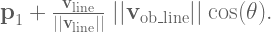
 vector to get the cosine of the angle, and then use
 rotated 90 degrees (the
  denoting outer product here). The way I’ve been thinking about this is basically taking your velocity vector,
  axis, and the bottom row by the difference along the
 instead of


 through
  . The 7th joint,
  , opens and closes the gripper, so we’re safe to ignore it in deriving our Jacobian. The arm segment lengths
  and
and  are named based on the nearest joint angles (makes easier reading in the Jacobian derivation).
 axis, so the rotational part of our transformation matrix
  is
is![^0_\textrm{org}\textbf{R} = \left[ \begin{array}{ccc} \textrm{cos}(q_0) & -\textrm{sin}(q_0) & 0 \\ \textrm{sin}(q_0) & \textrm{cos}(q_0) & 0 \\ 0 & 0 & 1 \end{array} \right],](https://s0.wp.com/latex.php?latex=%5E0_%5Ctextrm%7Borg%7D%5Ctextbf%7BR%7D+%3D+%5Cleft%5B+%5Cbegin%7Barray%7D%7Bccc%7D+%5Ctextrm%7Bcos%7D%28q_0%29+%26+-%5Ctextrm%7Bsin%7D%28q_0%29+%26+0+%5C%5C+%5Ctextrm%7Bsin%7D%28q_0%29+%26+%5Ctextrm%7Bcos%7D%28q_0%29+%26+0+%5C%5C+0+%26+0+%26+1+%5Cend%7Barray%7D+%5Cright%5D%2C&bg=ffffff&fg=555555&s=0&c=20201002)
![^0_\textrm{org}\textbf{D} = \left[ \begin{array}{c} 0 \\ 0 \\ 0 \end{array} \right].](https://s0.wp.com/latex.php?latex=%5E0_%5Ctextrm%7Borg%7D%5Ctextbf%7BD%7D+%3D+%5Cleft%5B+%5Cbegin%7Barray%7D%7Bc%7D+0+%5C%5C+0+%5C%5C+0+%5Cend%7Barray%7D+%5Cright%5D.&bg=ffffff&fg=555555&s=0&c=20201002)
![^0_\textrm{org}\textbf{T} = \left[ \begin{array}{cc} ^0_\textrm{org}\textbf{R} & ^0_\textrm{org}\textbf{D} \\ 0 & 1 \end{array} \right] = \left[ \begin{array}{cccc} \textrm{cos}(q_0) & -\textrm{sin}(q_0) & 0 & 0\\ \textrm{sin}(q_0) & \textrm{cos}(q_0) & 0 & 0 \\ 0 & 0 & 1 & 0 \\ 0 & 0 & 0 & 1 \end{array} \right] .](https://s0.wp.com/latex.php?latex=%5E0_%5Ctextrm%7Borg%7D%5Ctextbf%7BT%7D+%3D+%5Cleft%5B+%5Cbegin%7Barray%7D%7Bcc%7D+%5E0_%5Ctextrm%7Borg%7D%5Ctextbf%7BR%7D+%26+%5E0_%5Ctextrm%7Borg%7D%5Ctextbf%7BD%7D+%5C%5C+0+%26+1+%5Cend%7Barray%7D+%5Cright%5D+%3D+%5Cleft%5B+%5Cbegin%7Barray%7D%7Bcccc%7D+%5Ctextrm%7Bcos%7D%28q_0%29+%26+-%5Ctextrm%7Bsin%7D%28q_0%29+%26+0+%26+0%5C%5C+%5Ctextrm%7Bsin%7D%28q_0%29+%26+%5Ctextrm%7Bcos%7D%28q_0%29+%26+0+%26+0+%5C%5C+0+%26+0+%26+1+%26+0+%5C%5C+0+%26+0+%26+0+%26+1+%5Cend%7Barray%7D+%5Cright%5D+.&bg=ffffff&fg=555555&s=0&c=20201002)
 rotates around the
  . Our transformation matrix looks like
![^1_0\textbf{T} = \left[ \begin{array}{cccc} 1 & 0 & 0 & 0 \\ 0 & \textrm{cos}(q_1) & -\textrm{sin}(q_1) & l_1 \textrm{cos}(q_1) \\ 0 & \textrm{sin}(q_1) & \textrm{cos}(q_1) & l_1 \textrm{sin}(q_1) \\ 0 & 0 & 0 & 1 \end{array} \right] .](https://s0.wp.com/latex.php?latex=%5E1_0%5Ctextbf%7BT%7D+%3D+%5Cleft%5B+%5Cbegin%7Barray%7D%7Bcccc%7D+1+%26+0+%26+0+%26+0+%5C%5C+0+%26+%5Ctextrm%7Bcos%7D%28q_1%29+%26+-%5Ctextrm%7Bsin%7D%28q_1%29+%26+l_1+%5Ctextrm%7Bcos%7D%28q_1%29+%5C%5C+0+%26+%5Ctextrm%7Bsin%7D%28q_1%29+%26+%5Ctextrm%7Bcos%7D%28q_1%29+%26+l_1+%5Ctextrm%7Bsin%7D%28q_1%29+%5C%5C+0+%26+0+%26+0+%26+1+%5Cend%7Barray%7D+%5Cright%5D+.&bg=ffffff&fg=555555&s=0&c=20201002)
 also rotates around the
  . So our transformation matrix looks like
![^2_1\textbf{T} = \left[ \begin{array}{cccc} 1 & 0 & 0 & 0 \\ 0 & \textrm{cos}(q_2) & -\textrm{sin}(q_2) & 0 \\ 0 & \textrm{sin}(q_2) & \textrm{cos}(q_2) & 0 \\ 0 & 0 & 0 & 1 \end{array} \right] .](https://s0.wp.com/latex.php?latex=%5E2_1%5Ctextbf%7BT%7D+%3D+%5Cleft%5B+%5Cbegin%7Barray%7D%7Bcccc%7D+1+%26+0+%26+0+%26+0+%5C%5C+0+%26+%5Ctextrm%7Bcos%7D%28q_2%29+%26+-%5Ctextrm%7Bsin%7D%28q_2%29+%26+0+%5C%5C+0+%26+%5Ctextrm%7Bsin%7D%28q_2%29+%26+%5Ctextrm%7Bcos%7D%28q_2%29+%26+0+%5C%5C+0+%26+0+%26+0+%26+1+%5Cend%7Barray%7D+%5Cright%5D+.&bg=ffffff&fg=555555&s=0&c=20201002)
![^3_2\textbf{T} = \left[ \begin{array}{cccc} \textrm{cos}(q_3) & 0 & -\textrm{sin}(q_3) & 0\\ 0 & 1 & 0 & l_3 \\ \textrm{sin}(q_3) & 0 & \textrm{cos}(q_3) & 0\\ 0 & 0 & 0 & 1 \end{array} \right] .](https://s0.wp.com/latex.php?latex=%5E3_2%5Ctextbf%7BT%7D+%3D+%5Cleft%5B+%5Cbegin%7Barray%7D%7Bcccc%7D+%5Ctextrm%7Bcos%7D%28q_3%29+%26+0+%26+-%5Ctextrm%7Bsin%7D%28q_3%29+%26+0%5C%5C+0+%26+1+%26+0+%26+l_3+%5C%5C+%5Ctextrm%7Bsin%7D%28q_3%29+%26+0+%26+%5Ctextrm%7Bcos%7D%28q_3%29+%26+0%5C%5C+0+%26+0+%26+0+%26+1+%5Cend%7Barray%7D+%5Cright%5D+.&bg=ffffff&fg=555555&s=0&c=20201002)
 to
to ![^4_3\textbf{T} = \left[ \begin{array}{cccc} 1 & 0 & 0 & 0 \\ 0 & \textrm{cos}(q_4) & -\textrm{sin}(q_4) & 0 \\ 0 & \textrm{sin}(q_4) & \textrm{cos}(q_4) & 0 \\ 0 & 0 & 0 & 1 \end{array} \right] .](https://s0.wp.com/latex.php?latex=%5E4_3%5Ctextbf%7BT%7D+%3D+%5Cleft%5B+%5Cbegin%7Barray%7D%7Bcccc%7D+1+%26+0+%26+0+%26+0+%5C%5C+0+%26+%5Ctextrm%7Bcos%7D%28q_4%29+%26+-%5Ctextrm%7Bsin%7D%28q_4%29+%26+0+%5C%5C+0+%26+%5Ctextrm%7Bsin%7D%28q_4%29+%26+%5Ctextrm%7Bcos%7D%28q_4%29+%26+0+%5C%5C+0+%26+0+%26+0+%26+1+%5Cend%7Barray%7D+%5Cright%5D+.&bg=ffffff&fg=555555&s=0&c=20201002)
![^5_4\textbf{T} = \left[ \begin{array}{cccc} \textrm{cos}(q_5) & 0 & -\textrm{sin}(q_5) & 0 \\ 0 & 1 & 0 & l_5 \\ \textrm{sin}(q_5) & 0 & \textrm{cos}(q_5) & 0\\ 0 & 0 & 0 & 1 \end{array} \right] .](https://s0.wp.com/latex.php?latex=%5E5_4%5Ctextbf%7BT%7D+%3D+%5Cleft%5B+%5Cbegin%7Barray%7D%7Bcccc%7D+%5Ctextrm%7Bcos%7D%28q_5%29+%26+0+%26+-%5Ctextrm%7Bsin%7D%28q_5%29+%26+0+%5C%5C+0+%26+1+%26+0+%26+l_5+%5C%5C+%5Ctextrm%7Bsin%7D%28q_5%29+%26+0+%26+%5Ctextrm%7Bcos%7D%28q_5%29+%26+0%5C%5C+0+%26+0+%26+0+%26+1+%5Cend%7Barray%7D+%5Cright%5D+.&bg=ffffff&fg=555555&s=0&c=20201002)

 . This could be a big ol’ headache to do it by hand, OR we could use SymPy, the symbolic computation package for Python. Which is exactly what we’ll do. So after a quick
 to approximate applying torque that affects acceleration and then velocity.
 , get the Jacobian for the current state of the arm using the function above, find the set of joint torques to apply, approximate this control by generating a set of target joint angles to move to, and then repeat this whole loop until we’re within some threshold of the target position. Whew.
 trajectory of the hand, and the OSC will take care of turning the desired hand forces into torques that can be applied to the arm. All of the code used to generate the animations throughout this post can of course be found
 is the state of the DMP system,
 by a new term:
 .
. on the difference between the plant and DMP states.


![\textbf{J}(\textbf{q}) = \left[ \begin{array}{cc} -L_0 sin(q_0) - L_1 sin(q_0 + q_1) & -L_1 sin(q_0 + q_1) \\ L_0 cos(q_0) + L_1 cos(q_0 + q_1) & L_1 cos(q_0 + q_1) \end{array} \right].](https://s0.wp.com/latex.php?latex=%5Ctextbf%7BJ%7D%28%5Ctextbf%7Bq%7D%29+%3D+%5Cleft%5B+%5Cbegin%7Barray%7D%7Bcc%7D+-L_0+sin%28q_0%29+-+L_1+sin%28q_0+%2B+q_1%29+%26+-L_1+sin%28q_0+%2B+q_1%29+%5C%5C+L_0+cos%28q_0%29+%2B+L_1+cos%28q_0+%2B+q_1%29+%26+L_1+cos%28q_0+%2B+q_1%29+%5Cend%7Barray%7D+%5Cright%5D.&bg=ffffff&fg=555555&s=0&c=20201002)
 it can be that
  , so the Jacobian becomes
![\textbf{J}(\textbf{q}) = \left[ \begin{array}{cc} (L_0 + L_1)(-sin(q_0)) & -L_1 sin(q_0) \\ (L_0 + L_1) cos(q_0) & L_1 cos(q_0) \end{array} \right],](https://s0.wp.com/latex.php?latex=%5Ctextbf%7BJ%7D%28%5Ctextbf%7Bq%7D%29+%3D+%5Cleft%5B+%5Cbegin%7Barray%7D%7Bcc%7D+%28L_0+%2B+L_1%29%28-sin%28q_0%29%29+%26+-L_1+sin%28q_0%29+%5C%5C+%28L_0+%2B+L_1%29+cos%28q_0%29+%26+L_1+cos%28q_0%29+%5Cend%7Barray%7D+%5Cright%5D%2C&bg=ffffff&fg=555555&s=0&c=20201002)

 , where
  and
and  , the Jacobian is
![\textbf{J}(\textbf{q}) = \left[ \begin{array}{cc} -(L_0 - L_1) sin(q_0) & L_1 sin(q_0) \\ (L_0 + L_1) cos(q_0) & - L_1 cos(q_0) \end{array} \right].](https://s0.wp.com/latex.php?latex=%5Ctextbf%7BJ%7D%28%5Ctextbf%7Bq%7D%29+%3D+%5Cleft%5B+%5Cbegin%7Barray%7D%7Bcc%7D+-%28L_0+-+L_1%29+sin%28q_0%29+%26+L_1+sin%28q_0%29+%5C%5C+%28L_0+%2B+L_1%29+cos%28q_0%29+%26+-+L_1+cos%28q_0%29+%5Cend%7Barray%7D+%5Cright%5D.&bg=ffffff&fg=555555&s=0&c=20201002)

 can be found instead.
 is found. To get the inverse of this matrix (i.e. to find
  ) from the returned
  and
and  matrices is a matter of inverting the matrix
  :
:

 and the control signal from the secondary controller
  . Define the force to apply to the system
 is the pseudo-inverse of
  .
.
![\ddot{\textbf{x}} = \textbf{J}_{ee}(\textbf{q}) \textbf{M}^{-1}(\textbf{q}) [\textbf{J}_{ee}^T(\textbf{q}) \; \textbf{M}_{\textbf{x}_{ee}}(\textbf{q}) \; \ddot{\textbf{x}}_\textrm{des} - (\textbf{I} - \textbf{J}_{ee}^T(\textbf{q})\;\textbf{J}_{ee}^{T+}(\textbf{q}))\;\textbf{u}_{\textrm{null}}].](https://s0.wp.com/latex.php?latex=%5Cddot%7B%5Ctextbf%7Bx%7D%7D+%3D+%5Ctextbf%7BJ%7D_%7Bee%7D%28%5Ctextbf%7Bq%7D%29+%5Ctextbf%7BM%7D%5E%7B-1%7D%28%5Ctextbf%7Bq%7D%29+%5B%5Ctextbf%7BJ%7D_%7Bee%7D%5ET%28%5Ctextbf%7Bq%7D%29+%5C%3B+%5Ctextbf%7BM%7D_%7B%5Ctextbf%7Bx%7D_%7Bee%7D%7D%28%5Ctextbf%7Bq%7D%29+%5C%3B+%5Cddot%7B%5Ctextbf%7Bx%7D%7D_%5Ctextrm%7Bdes%7D+-+%28%5Ctextbf%7BI%7D+-+%5Ctextbf%7BJ%7D_%7Bee%7D%5ET%28%5Ctextbf%7Bq%7D%29%5C%3B%5Ctextbf%7BJ%7D_%7Bee%7D%5E%7BT%2B%7D%28%5Ctextbf%7Bq%7D%29%29%5C%3B%5Ctextbf%7Bu%7D_%7B%5Ctextrm%7Bnull%7D%7D%5D.&bg=ffffff&fg=555555&s=0&c=20201002)
![\ddot{\textbf{x}} = \textbf{J}_{ee}(\textbf{q}) \textbf{M}^{-1}(\textbf{q}) \textbf{J}_{ee}^T(\textbf{q}) \; \textbf{M}_{\textbf{x}_{ee}}(\textbf{q}) \; \ddot{\textbf{x}}_\textrm{des} - \textbf{J}_{ee}(\textbf{q}) \textbf{M}^{-1}(\textbf{q})[\textbf{I} - \textbf{J}_{ee}^T(\textbf{q})\;\textbf{J}_{ee}^{T+}(\textbf{q})]\;\textbf{u}_{\textrm{null}},](https://s0.wp.com/latex.php?latex=%5Cddot%7B%5Ctextbf%7Bx%7D%7D+%3D+%5Ctextbf%7BJ%7D_%7Bee%7D%28%5Ctextbf%7Bq%7D%29+%5Ctextbf%7BM%7D%5E%7B-1%7D%28%5Ctextbf%7Bq%7D%29+%5Ctextbf%7BJ%7D_%7Bee%7D%5ET%28%5Ctextbf%7Bq%7D%29+%5C%3B+%5Ctextbf%7BM%7D_%7B%5Ctextbf%7Bx%7D_%7Bee%7D%7D%28%5Ctextbf%7Bq%7D%29+%5C%3B+%5Cddot%7B%5Ctextbf%7Bx%7D%7D_%5Ctextrm%7Bdes%7D+-+%5Ctextbf%7BJ%7D_%7Bee%7D%28%5Ctextbf%7Bq%7D%29+%5Ctextbf%7BM%7D%5E%7B-1%7D%28%5Ctextbf%7Bq%7D%29%5B%5Ctextbf%7BI%7D+-+%5Ctextbf%7BJ%7D_%7Bee%7D%5ET%28%5Ctextbf%7Bq%7D%29%5C%3B%5Ctextbf%7BJ%7D_%7Bee%7D%5E%7BT%2B%7D%28%5Ctextbf%7Bq%7D%29%5D%5C%3B%5Ctextbf%7Bu%7D_%7B%5Ctextrm%7Bnull%7D%7D%2C+&bg=ffffff&fg=555555&s=0&c=20201002)
![\textbf{J}_{ee}(\textbf{q})\textbf{M}^{-1}(\textbf{q}) [\textbf{I} - \textbf{J}_{ee}^T (\textbf{q})\textbf{J}_{ee}^{T+}(\textbf{q})] \textbf{u}_{\textrm{null}} = \textbf{0},](https://s0.wp.com/latex.php?latex=%5Ctextbf%7BJ%7D_%7Bee%7D%28%5Ctextbf%7Bq%7D%29%5Ctextbf%7BM%7D%5E%7B-1%7D%28%5Ctextbf%7Bq%7D%29+%5B%5Ctextbf%7BI%7D+-+%5Ctextbf%7BJ%7D_%7Bee%7D%5ET+%28%5Ctextbf%7Bq%7D%29%5Ctextbf%7BJ%7D_%7Bee%7D%5E%7BT%2B%7D%28%5Ctextbf%7Bq%7D%29%5D+%5Ctextbf%7Bu%7D_%7B%5Ctextrm%7Bnull%7D%7D+%3D+%5Ctextbf%7B0%7D%2C&bg=ffffff&fg=555555&s=0&c=20201002)
![\textbf{J}_{ee} (\textbf{q}) \; \textbf{M}^{-1}(\textbf{q}) [\textbf{1} - \textbf{J}_{ee}^T (\textbf{q}) \; \textbf{J}_{ee}^{T+} (\textbf{q})] = \textbf{0},](https://s0.wp.com/latex.php?latex=%5Ctextbf%7BJ%7D_%7Bee%7D+%28%5Ctextbf%7Bq%7D%29+%5C%3B+%5Ctextbf%7BM%7D%5E%7B-1%7D%28%5Ctextbf%7Bq%7D%29+%5B%5Ctextbf%7B1%7D+-+%5Ctextbf%7BJ%7D_%7Bee%7D%5ET+%28%5Ctextbf%7Bq%7D%29+%5C%3B+%5Ctextbf%7BJ%7D_%7Bee%7D%5E%7BT%2B%7D+%28%5Ctextbf%7Bq%7D%29%5D+%3D+%5Ctextbf%7B0%7D%2C&bg=ffffff&fg=555555&s=0&c=20201002)


 plane, shown below:
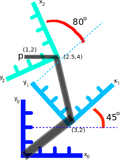
![\textbf{q} = [q_0, q_1, q_2]^T](https://s0.wp.com/latex.php?latex=%5Ctextbf%7Bq%7D+%3D+%5Bq_0%2C+q_1%2C+q_2%5D%5ET&bg=ffffff&fg=555555&s=0&c=20201002) with default positions
with default positions ![\textbf{q}^0 = \left[\frac{\pi}{3}, \frac{\pi}{4}, \frac{\pi}{4} \right]^T](https://s0.wp.com/latex.php?latex=%5Ctextbf%7Bq%7D%5E0+%3D+%5Cleft%5B%5Cfrac%7B%5Cpi%7D%7B3%7D%2C+%5Cfrac%7B%5Cpi%7D%7B4%7D%2C+%5Cfrac%7B%5Cpi%7D%7B4%7D+%5Cright%5D%5ET&bg=ffffff&fg=555555&s=0&c=20201002) . The control signal of the secondary controller is the difference between the target state and the current system state
. The control signal of the secondary controller is the difference between the target state and the current system state
 is a gain term.
![\textrm{com}_0 = \left[ \begin{array}{c} \frac{1}{2}cos(q_0) \\ 0 \\ \frac{1}{2}sin(q_0) \end{array} \right], \;\;\;\; \textrm{com}_1 = \left[ \begin{array}{c} \frac{1}{4}cos(q_1) \\ 0 \\ \frac{1}{4}sin(q_1) \end{array} \right] \;\;\;\; \textrm{com}_2 = \left[ \begin{array}{c} \frac{1}{2}cos(q_2) \\ 0 \\ \frac{1}{4} sin (q_2) \end{array} \right],](https://s0.wp.com/latex.php?latex=%5Ctextrm%7Bcom%7D_0+%3D+%5Cleft%5B+%5Cbegin%7Barray%7D%7Bc%7D+%5Cfrac%7B1%7D%7B2%7Dcos%28q_0%29+%5C%5C+0+%5C%5C+%5Cfrac%7B1%7D%7B2%7Dsin%28q_0%29+%5Cend%7Barray%7D+%5Cright%5D%2C+%5C%3B%5C%3B%5C%3B%5C%3B+%5Ctextrm%7Bcom%7D_1+%3D+%5Cleft%5B+%5Cbegin%7Barray%7D%7Bc%7D+%5Cfrac%7B1%7D%7B4%7Dcos%28q_1%29+%5C%5C+0+%5C%5C+%5Cfrac%7B1%7D%7B4%7Dsin%28q_1%29+%5Cend%7Barray%7D+%5Cright%5D+%5C%3B%5C%3B%5C%3B%5C%3B+%5Ctextrm%7Bcom%7D_2+%3D+%5Cleft%5B+%5Cbegin%7Barray%7D%7Bc%7D+%5Cfrac%7B1%7D%7B2%7Dcos%28q_2%29+%5C%5C+0+%5C%5C+%5Cfrac%7B1%7D%7B4%7D+sin+%28q_2%29+%5Cend%7Barray%7D+%5Cright%5D%2C&bg=ffffff&fg=555555&s=0&c=20201002)
![\textbf{J}_0(\textbf{q}) = \left[ \begin{array}{ccc} -\frac{1}{2} sin(q_0) & 0 & 0 \\ 0 & 0 & 0 \\ \frac{1}{2} cos(q_0) & 0 & 0 \\ 0 & 0 & 0 \\ 1 & 0 & 0 \\ 0 & 0 & 0 \end{array} \right],](https://s0.wp.com/latex.php?latex=%5Ctextbf%7BJ%7D_0%28%5Ctextbf%7Bq%7D%29+%3D+%5Cleft%5B+%5Cbegin%7Barray%7D%7Bccc%7D+-%5Cfrac%7B1%7D%7B2%7D+sin%28q_0%29+%26+0+%26+0+%5C%5C+0+%26+0+%26+0+%5C%5C+%5Cfrac%7B1%7D%7B2%7D+cos%28q_0%29+%26+0+%26+0+%5C%5C+0+%26+0+%26+0+%5C%5C+1+%26+0+%26+0+%5C%5C+0+%26+0+%26+0+%5Cend%7Barray%7D+%5Cright%5D%2C&bg=ffffff&fg=555555&s=0&c=20201002)
![\textbf{J}_1(\textbf{q}) = \left[ \begin{array}{ccc} -L_0sin(q_0) - \frac{1}{4}sin(q_{01}) & -\frac{1}{4}sin(q_{01}) & 0 \\ 0 & 0 & 0 \\ L_0 cos(q_0) + \frac{1}{4} cos(q_{01})& \frac{1}{4} cos(q_{01}) & 0 \\ 0 & 0 & 0 \\ 1 & 1 & 0 \\ 0 & 0 & 0 \end{array} \right]](https://s0.wp.com/latex.php?latex=%5Ctextbf%7BJ%7D_1%28%5Ctextbf%7Bq%7D%29+%3D+%5Cleft%5B+%5Cbegin%7Barray%7D%7Bccc%7D+-L_0sin%28q_0%29+-+%5Cfrac%7B1%7D%7B4%7Dsin%28q_%7B01%7D%29+%26+-%5Cfrac%7B1%7D%7B4%7Dsin%28q_%7B01%7D%29+%26+0+%5C%5C+0+%26+0+%26+0+%5C%5C+L_0+cos%28q_0%29+%2B+%5Cfrac%7B1%7D%7B4%7D+cos%28q_%7B01%7D%29%26+%5Cfrac%7B1%7D%7B4%7D+cos%28q_%7B01%7D%29+%26+0+%5C%5C+0+%26+0+%26+0+%5C%5C+1+%26+1+%26+0+%5C%5C+0+%26+0+%26+0+%5Cend%7Barray%7D+%5Cright%5D&bg=ffffff&fg=555555&s=0&c=20201002)
![\textbf{J}_2(\textbf{q}) = \left[ \begin{array}{ccc} -L_0sin(q_0) - L_1sin(q_{01}) - \frac{1}{2}sin(q_{012}) & -L_1sin(q_{01}) - \frac{1}{2}sin(q_{012}) & - \frac{1}{2}sin(q_{012}) \\ 0 & 0 & 0 \\ L_0 cos(q_0) + L_1 cos(q_{01}) + \frac{1}{4}cos(q_{012}) & L_1 cos(q_{01}) + \frac{1}{4} cos(q_{012}) & \frac{1}{4}cos(q_{012}) \\ 0 & 0 & 0 \\ 1 & 1 & 1 \\ 0 & 0 & 0 \end{array} \right].](https://s0.wp.com/latex.php?latex=%5Ctextbf%7BJ%7D_2%28%5Ctextbf%7Bq%7D%29+%3D+%5Cleft%5B+%5Cbegin%7Barray%7D%7Bccc%7D+-L_0sin%28q_0%29+-+L_1sin%28q_%7B01%7D%29+-+%5Cfrac%7B1%7D%7B2%7Dsin%28q_%7B012%7D%29+%26+-L_1sin%28q_%7B01%7D%29+-+%5Cfrac%7B1%7D%7B2%7Dsin%28q_%7B012%7D%29+%26+-+%5Cfrac%7B1%7D%7B2%7Dsin%28q_%7B012%7D%29+%5C%5C+0+%26+0+%26+0+%5C%5C+L_0+cos%28q_0%29+%2B+L_1+cos%28q_%7B01%7D%29+%2B+%5Cfrac%7B1%7D%7B4%7Dcos%28q_%7B012%7D%29+%26+L_1+cos%28q_%7B01%7D%29+%2B+%5Cfrac%7B1%7D%7B4%7D+cos%28q_%7B012%7D%29+%26+%5Cfrac%7B1%7D%7B4%7Dcos%28q_%7B012%7D%29+%5C%5C+0+%26+0+%26+0+%5C%5C+1+%26+1+%26+1+%5C%5C+0+%26+0+%26+0+%5Cend%7Barray%7D+%5Cright%5D.&bg=ffffff&fg=555555&s=0&c=20201002)
![\textbf{J}_{ee} = \left[ \begin{array}{ccc} -L_0 sin(q_0) - L_1 sin(q_{01}) - L_2 sin(q_{012}) & - L_1 sin(q_{01}) - L_2 sin(q_{012}) & - L_2 sin(q_{012}) \\ L_0 cos(q_0) + L_1 cos(q_{01}) + L_2 cos(q_{012}) & L_1 cos(q_{01}) + L_2 cos(q_{012}) & L_2 cos(q_{012}), \end{array} \right]](https://s0.wp.com/latex.php?latex=%5Ctextbf%7BJ%7D_%7Bee%7D+%3D+%5Cleft%5B+%5Cbegin%7Barray%7D%7Bccc%7D+-L_0+sin%28q_0%29+-+L_1+sin%28q_%7B01%7D%29+-+L_2+sin%28q_%7B012%7D%29+%26+-+L_1+sin%28q_%7B01%7D%29+-+L_2+sin%28q_%7B012%7D%29+%26+-+L_2+sin%28q_%7B012%7D%29+%5C%5C+L_0+cos%28q_0%29+%2B+L_1+cos%28q_%7B01%7D%29+%2B+L_2+cos%28q_%7B012%7D%29+%26+L_1+cos%28q_%7B01%7D%29+%2B+L_2+cos%28q_%7B012%7D%29+%26+L_2+cos%28q_%7B012%7D%29%2C+%5Cend%7Barray%7D+%5Cright%5D&bg=ffffff&fg=555555&s=0&c=20201002)
 and
and  .
.![\textbf{u} = \textbf{J}^T_{ee}(\textbf{q}) \; \textbf{M}_{\textbf{x}_{ee}}(\textbf{q}) [k_p (\textbf{x}_{\textrm{des}} - \textbf{x}) + k_v (\dot{\textbf{x}}_{\textrm{des}} - \dot{\textbf{x}})] - \textbf{g}(\textbf{q}),](https://s0.wp.com/latex.php?latex=%5Ctextbf%7Bu%7D+%3D+%5Ctextbf%7BJ%7D%5ET_%7Bee%7D%28%5Ctextbf%7Bq%7D%29+%5C%3B+%5Ctextbf%7BM%7D_%7B%5Ctextbf%7Bx%7D_%7Bee%7D%7D%28%5Ctextbf%7Bq%7D%29+%5Bk_p+%28%5Ctextbf%7Bx%7D_%7B%5Ctextrm%7Bdes%7D%7D+-+%5Ctextbf%7Bx%7D%29+%2B+k_v+%28%5Cdot%7B%5Ctextbf%7Bx%7D%7D_%7B%5Ctextrm%7Bdes%7D%7D+-+%5Cdot%7B%5Ctextbf%7Bx%7D%7D%29%5D+-+%5Ctextbf%7Bg%7D%28%5Ctextbf%7Bq%7D%29%2C&bg=ffffff&fg=555555&s=0&c=20201002)
 was defined
  is defined
  , and adding in the null space control signal and filter gives
![\textbf{u} = \textbf{J}^T_{ee}(\textbf{q}) \; \textbf{M}_{\textbf{x}_{ee}}(\textbf{q}) [k_p (\textbf{x}_{\textrm{des}} - \textbf{x}) + k_v (\dot{\textbf{x}}_{\textrm{des}} - \dot{\textbf{x}})] - (\textbf{I} - \textbf{J}^T_{ee}(\textbf{q}) \textbf{J}^{T+}_{ee}(\textbf{q})) \textbf{u}_{\textrm{null}} - \textbf{g}(\textbf{q}),](https://s0.wp.com/latex.php?latex=%5Ctextbf%7Bu%7D+%3D+%5Ctextbf%7BJ%7D%5ET_%7Bee%7D%28%5Ctextbf%7Bq%7D%29+%5C%3B+%5Ctextbf%7BM%7D_%7B%5Ctextbf%7Bx%7D_%7Bee%7D%7D%28%5Ctextbf%7Bq%7D%29+%5Bk_p+%28%5Ctextbf%7Bx%7D_%7B%5Ctextrm%7Bdes%7D%7D+-+%5Ctextbf%7Bx%7D%29+%2B+k_v+%28%5Cdot%7B%5Ctextbf%7Bx%7D%7D_%7B%5Ctextrm%7Bdes%7D%7D+-+%5Cdot%7B%5Ctextbf%7Bx%7D%7D%29%5D+-+%28%5Ctextbf%7BI%7D+-+%5Ctextbf%7BJ%7D%5ET_%7Bee%7D%28%5Ctextbf%7Bq%7D%29+%5Ctextbf%7BJ%7D%5E%7BT%2B%7D_%7Bee%7D%28%5Ctextbf%7Bq%7D%29%29+%5Ctextbf%7Bu%7D_%7B%5Ctextrm%7Bnull%7D%7D+-+%5Ctextbf%7Bg%7D%28%5Ctextbf%7Bq%7D%29%2C&bg=ffffff&fg=555555&s=0&c=20201002)
 is the dynamically consistent generalized inverse defined above, and
![\textbf{J} = \left[ \begin{array}{cc} -L_0 sin(\theta_0) - L_1 sin(\theta_0 + \theta_1) & - L_1 sin(\theta_0 + \theta_1) \\ L_0 cos(\theta_0) + L_1 cos(\theta_0 + \theta_1) & L_1 cos(\theta_0 + \theta_1) \\ 0 & 0 \\ 0 & 0 \\ 0 & 0 \\ 1 & 1 \end{array} \right]](https://s0.wp.com/latex.php?latex=%5Ctextbf%7BJ%7D+%3D+%5Cleft%5B+%5Cbegin%7Barray%7D%7Bcc%7D+-L_0+sin%28%5Ctheta_0%29+-+L_1+sin%28%5Ctheta_0+%2B+%5Ctheta_1%29+%26+-+L_1+sin%28%5Ctheta_0+%2B+%5Ctheta_1%29+%5C%5C+L_0+cos%28%5Ctheta_0%29+%2B+L_1+cos%28%5Ctheta_0+%2B+%5Ctheta_1%29+%26+L_1+cos%28%5Ctheta_0+%2B+%5Ctheta_1%29+%5C%5C+0+%26+0+%5C%5C+0+%26+0+%5C%5C+0+%26+0+%5C%5C+1+%26+1+%5Cend%7Barray%7D+%5Cright%5D&bg=ffffff&fg=555555&s=0&c=20201002)
 , we can go ahead and transform forces from end-effector (hand) space to joint space as we discussed in
 as its component parts
 is end-effector acceleration, and
  is the inertia matrix in operational space. Unfortunately, this isn’t just the normal inertia matrix, so let’s take a look here at how to go about deriving it.
 allows inertia to be cancelled out in joint-space by incorporating it into the control signal, but to cancel out the inertia of the system in operational space more work is still required. The first step will be calculating the acceleration in operational space. This can be found by taking the time derivative of our original Jacobian equation.
![\ddot{\textbf{x}} = \dot{\textbf{J}}_{ee}(\textbf{q}) \; \dot{\textbf{q}} + \textbf{J}_{ee} (\textbf{q})\; \textbf{M}^{-1}(\textbf{q}) [ \textbf{u} - \textbf{C}(\textbf{q}, \dot{\textbf{q}})].](https://s0.wp.com/latex.php?latex=%5Cddot%7B%5Ctextbf%7Bx%7D%7D+%3D+%5Cdot%7B%5Ctextbf%7BJ%7D%7D_%7Bee%7D%28%5Ctextbf%7Bq%7D%29+%5C%3B+%5Cdot%7B%5Ctextbf%7Bq%7D%7D+%2B+%5Ctextbf%7BJ%7D_%7Bee%7D+%28%5Ctextbf%7Bq%7D%29%5C%3B+%5Ctextbf%7BM%7D%5E%7B-1%7D%28%5Ctextbf%7Bq%7D%29+%5B+%5Ctextbf%7Bu%7D+-+%5Ctextbf%7BC%7D%28%5Ctextbf%7Bq%7D%2C+%5Cdot%7B%5Ctextbf%7Bq%7D%7D%29%5D.+&bg=ffffff&fg=555555&s=0&c=20201002)

 denotes the desired end-effector acceleration. Substituting the above equation into our equation for acceleration in operational space gives
![\ddot{\textbf{x}} = \dot{\textbf{J}}_{ee}(\textbf{q}) \; \dot{\textbf{q}} + \textbf{J}_{ee} (\textbf{q})\; \textbf{M}^{-1}(\textbf{q}) [ \textbf{J}_{ee}^T(\textbf{q})\; \textbf{M}_{\textbf{x}_{ee}}(\textbf{q})\; \ddot{\textbf{x}}_\textrm{des} - \textbf{C}(\textbf{q}, \dot{\textbf{q}})].](https://s0.wp.com/latex.php?latex=%5Cddot%7B%5Ctextbf%7Bx%7D%7D+%3D+%5Cdot%7B%5Ctextbf%7BJ%7D%7D_%7Bee%7D%28%5Ctextbf%7Bq%7D%29+%5C%3B+%5Cdot%7B%5Ctextbf%7Bq%7D%7D+%2B+%5Ctextbf%7BJ%7D_%7Bee%7D+%28%5Ctextbf%7Bq%7D%29%5C%3B+%5Ctextbf%7BM%7D%5E%7B-1%7D%28%5Ctextbf%7Bq%7D%29+%5B+%5Ctextbf%7BJ%7D_%7Bee%7D%5ET%28%5Ctextbf%7Bq%7D%29%5C%3B+%5Ctextbf%7BM%7D_%7B%5Ctextbf%7Bx%7D_%7Bee%7D%7D%28%5Ctextbf%7Bq%7D%29%5C%3B+%5Cddot%7B%5Ctextbf%7Bx%7D%7D_%5Ctextrm%7Bdes%7D+-+%5Ctextbf%7BC%7D%28%5Ctextbf%7Bq%7D%2C+%5Cdot%7B%5Ctextbf%7Bq%7D%7D%29%5D.&bg=ffffff&fg=555555&s=0&c=20201002)
![\ddot{\textbf{x}} = \textbf{J}_{ee}(\textbf{q})\; \textbf{M}^{-1}(\textbf{q}) \; \textbf{J}_{ee}^T(\textbf{q})\; \textbf{M}_{\textbf{x}_{ee}}(\textbf{q})\; \ddot{\textbf{x}}_\textrm{des} + [\dot{\textbf{J}}_{ee}(\textbf{q}) \; \dot{\textbf{q}} - \textbf{J}_{ee}(\textbf{q})\textbf{M}^{-1}(\textbf{q}) \; \textbf{C}(\textbf{q}, \dot{\textbf{q}})],](https://s0.wp.com/latex.php?latex=%5Cddot%7B%5Ctextbf%7Bx%7D%7D+%3D+%5Ctextbf%7BJ%7D_%7Bee%7D%28%5Ctextbf%7Bq%7D%29%5C%3B+%5Ctextbf%7BM%7D%5E%7B-1%7D%28%5Ctextbf%7Bq%7D%29+%5C%3B+%5Ctextbf%7BJ%7D_%7Bee%7D%5ET%28%5Ctextbf%7Bq%7D%29%5C%3B+%5Ctextbf%7BM%7D_%7B%5Ctextbf%7Bx%7D_%7Bee%7D%7D%28%5Ctextbf%7Bq%7D%29%5C%3B+%5Cddot%7B%5Ctextbf%7Bx%7D%7D_%5Ctextrm%7Bdes%7D+%2B+%5B%5Cdot%7B%5Ctextbf%7BJ%7D%7D_%7Bee%7D%28%5Ctextbf%7Bq%7D%29+%5C%3B+%5Cdot%7B%5Ctextbf%7Bq%7D%7D+-+%5Ctextbf%7BJ%7D_%7Bee%7D%28%5Ctextbf%7Bq%7D%29%5Ctextbf%7BM%7D%5E%7B-1%7D%28%5Ctextbf%7Bq%7D%29+%5C%3B+%5Ctextbf%7BC%7D%28%5Ctextbf%7Bq%7D%2C+%5Cdot%7B%5Ctextbf%7Bq%7D%7D%29%5D%2C+&bg=ffffff&fg=555555&s=0&c=20201002)

 needs to be chosen carefully. By setting
![\textbf{M}_{\textbf{x}_{ee}}(\textbf{q}) = [\textbf{J}_{ee}(\textbf{q}) \; \textbf{M}^{-1}(\textbf{q}) \; \textbf{J}_{ee}^T(\textbf{q})]^{-1},](https://s0.wp.com/latex.php?latex=%5Ctextbf%7BM%7D_%7B%5Ctextbf%7Bx%7D_%7Bee%7D%7D%28%5Ctextbf%7Bq%7D%29+%3D+%5B%5Ctextbf%7BJ%7D_%7Bee%7D%28%5Ctextbf%7Bq%7D%29+%5C%3B+%5Ctextbf%7BM%7D%5E%7B-1%7D%28%5Ctextbf%7Bq%7D%29+%5C%3B+%5Ctextbf%7BJ%7D_%7Bee%7D%5ET%28%5Ctextbf%7Bq%7D%29%5D%5E%7B-1%7D%2C&bg=ffffff&fg=555555&s=0&c=20201002)
![\ddot{\textbf{x}} = \textbf{J}_{ee}(\textbf{q})\; \textbf{M}^{-1}(\textbf{q}) \textbf{J}_{ee}^T(\textbf{q})\; [\textbf{J}_{ee}(\textbf{q}) \; \textbf{M}^{-1}(\textbf{q}) \; \textbf{J}_{ee}^T(\textbf{q})]^{-1} \; \ddot{\textbf{x}}_\textrm{des},](https://s0.wp.com/latex.php?latex=%5Cddot%7B%5Ctextbf%7Bx%7D%7D+%3D+%5Ctextbf%7BJ%7D_%7Bee%7D%28%5Ctextbf%7Bq%7D%29%5C%3B+%5Ctextbf%7BM%7D%5E%7B-1%7D%28%5Ctextbf%7Bq%7D%29+%5Ctextbf%7BJ%7D_%7Bee%7D%5ET%28%5Ctextbf%7Bq%7D%29%5C%3B+%5B%5Ctextbf%7BJ%7D_%7Bee%7D%28%5Ctextbf%7Bq%7D%29+%5C%3B+%5Ctextbf%7BM%7D%5E%7B-1%7D%28%5Ctextbf%7Bq%7D%29+%5C%3B+%5Ctextbf%7BJ%7D_%7Bee%7D%5ET%28%5Ctextbf%7Bq%7D%29%5D%5E%7B-1%7D+%5C%3B+%5Cddot%7B%5Ctextbf%7Bx%7D%7D_%5Ctextrm%7Bdes%7D%2C&bg=ffffff&fg=555555&s=0&c=20201002)


![\textbf{u} = \textbf{J}_{ee}^T(\textbf{q}) \; \textbf{M}_{\textbf{x}_{ee}}(\textbf{q}) [k_p (\textbf{x}_{\textrm{des}} - \textbf{x}) + k_v (\dot{\textbf{x}}_{\textrm{des}} - \dot{\textbf{x}})] + \textbf{g}(\textbf{q}).](https://s0.wp.com/latex.php?latex=%5Ctextbf%7Bu%7D+%3D+%5Ctextbf%7BJ%7D_%7Bee%7D%5ET%28%5Ctextbf%7Bq%7D%29+%5C%3B+%5Ctextbf%7BM%7D_%7B%5Ctextbf%7Bx%7D_%7Bee%7D%7D%28%5Ctextbf%7Bq%7D%29+%5Bk_p+%28%5Ctextbf%7Bx%7D_%7B%5Ctextrm%7Bdes%7D%7D+-+%5Ctextbf%7Bx%7D%29+%2B+k_v+%28%5Cdot%7B%5Ctextbf%7Bx%7D%7D_%7B%5Ctextrm%7Bdes%7D%7D+-+%5Cdot%7B%5Ctextbf%7Bx%7D%7D%29%5D+%2B+%5Ctextbf%7Bg%7D%28%5Ctextbf%7Bq%7D%29.&bg=ffffff&fg=555555&s=0&c=20201002)
