Robot control part 4: Operation space control

In this post we’ll look at operational space control and how to derive the control equations. I’d like to mention again that these posts have all come about as a result of me reading and working through Samir Menon’s operational space control tutorial, where he works through an implementation example on a revolute-prismatic-prismatic robot arm.

Generalized coordinates vs operational space

The term generalized coordinates refers to a characterization of the system that uniquely defines its configuration. For example, if our robot has 7 degrees of freedom, then there are 7 state variables, such that when all these variables are given we can fully account for the position of the robot. In the previous posts of this series we’ve been describing robotic arms in joint space, and for these systems joint space is an example of generalized coordinates. This means that if we know the angles of all of the joints, we can draw out exactly what position that robot is in. An example of a coordinate system that does not uniquely define the configuration of a robotic arm would be one that describes only the $x$ position of the end-effector.

So generalized coordinates tell us everything we need to know about where the robot is, that’s great. The problem with generalized coordinates, though, is that planning trajectories in this space for tasks that we’re interested in performing tends not to be straight forward. For example, if we have a robotic arm, and we want to control the position of the end-effector, it’s not obvious how to control the position of the end-effector by specifying a trajectory for each of the arm’s joints to follow through joint space.

The idea behind operational space control is to abstract away from the generalized coordinates of the system and plan a trajectory in a coordinate system that is directly relevant to the task that we wish to perform. Going back to the common end-effector position control situation, we would like to operate our arm in 3D $(x,y,z)$ Cartesian space. In this space, it’s obvious what trajectory to follow to move the end-effector between two positions (most of the time it will just be a straight line in each dimension). So our goal is to build a control system that lets us specify a trajectory in our task space and will transform this signal into generalized coordinates that it can then send out to the system for execution.

Operational space control of simple robot arm

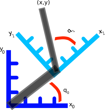
Alright, we’re going to work through an example. The generalized coordinates for this example is going to be joint space, and the operational space is going to be the end-effector Cartesian coordinates relative to the a reference frame attached to the base. Recycling the robot from the second post in this series, here’s the set up we’ll be working with:

Once again, we’re going to need to find the Jacobians for the end-effector of the robot. Fortunately, we’ve already done this:

$\textbf{J} = \left[ \begin{array}{cc} -L_0 sin(\theta_0) - L_1 sin(\theta_0 + \theta_1) & - L_1 sin(\theta_0 + \theta_1) \\ L_0 cos(\theta_0) + L_1 cos(\theta_0 + \theta_1) & L_1 cos(\theta_0 + \theta_1) \\ 0 & 0 \\ 0 & 0 \\ 0 & 0 \\ 1 & 1 \end{array} \right]$

Great! So now that we have $\textbf{J}$ , we can go ahead and transform forces from end-effector (hand) space to joint space as we discussed in the second post:

$\textbf{u} = \textbf{J}_{ee}^T(\textbf{q}) \; \textbf{F}_{\textbf{x}}.$

Rewriting $\textbf{F}_\textbf{x}$ as its component parts

$\textbf{F}_{\textbf{x}} = \textbf{M}_{\textbf{x}_{ee}}(\textbf{q}) \; \ddot{\textbf{x}}_\textrm{des},$

where $\ddot{\textbf{x}}$ is end-effector acceleration, and $\textbf{M}_{\textbf{x}_{ee}(\textbf{q})}$ is the inertia matrix in operational space. Unfortunately, this isn’t just the normal inertia matrix, so let’s take a look here at how to go about deriving it.

Inertia in operational space

Being able to calculate $\textbf{M}(\textbf{q})$ allows inertia to be cancelled out in joint-space by incorporating it into the control signal, but to cancel out the inertia of the system in operational space more work is still required. The first step will be calculating the acceleration in operational space. This can be found by taking the time derivative of our original Jacobian equation.

$\frac{d}{d t}\dot{\textbf{x}} = \frac{d}{d t} (\textbf{J}_{ee}(\textbf{q}) \; \dot{\textbf{q}}),$

$\ddot{\textbf{x}} = \dot{\textbf{J}}_{ee}(\textbf{q}) \; \dot{\textbf{q}} + \textbf{J}_{ee} (\textbf{q})\; \ddot{\textbf{q}}.$

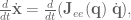
Substituting in the dynamics of the system, as defined in the previous post, but ignoring the effects of gravity for now, gives:

$\ddot{\textbf{x}} = \dot{\textbf{J}}_{ee}(\textbf{q}) \; \dot{\textbf{q}} + \textbf{J}_{ee} (\textbf{q})\; \textbf{M}^{-1}(\textbf{q}) [ \textbf{u} - \textbf{C}(\textbf{q}, \dot{\textbf{q}})].$

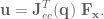
Define the control signal

$\textbf{u} = \textbf{J}_{ee}^T(\textbf{q}) \textbf{F}_\textbf{x},$

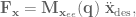
where substituting in for $\textbf{F}_\textbf{x}$ , the desired end-effector force, gives

$\textbf{u} = \textbf{J}_{ee}^T(\textbf{q})\; \textbf{M}_{\textbf{x}_{ee}}(\textbf{q})\; \ddot{\textbf{x}}_\textrm{des},$

where $\ddot{\textbf{x}}_\textrm{des}$ denotes the desired end-effector acceleration. Substituting the above equation into our equation for acceleration in operational space gives

$\ddot{\textbf{x}} = \dot{\textbf{J}}_{ee}(\textbf{q}) \; \dot{\textbf{q}} + \textbf{J}_{ee} (\textbf{q})\; \textbf{M}^{-1}(\textbf{q}) [ \textbf{J}_{ee}^T(\textbf{q})\; \textbf{M}_{\textbf{x}_{ee}}(\textbf{q})\; \ddot{\textbf{x}}_\textrm{des} - \textbf{C}(\textbf{q}, \dot{\textbf{q}})].$

Rearranging terms leads to

$\ddot{\textbf{x}} = \textbf{J}_{ee}(\textbf{q})\; \textbf{M}^{-1}(\textbf{q}) \; \textbf{J}_{ee}^T(\textbf{q})\; \textbf{M}_{\textbf{x}_{ee}}(\textbf{q})\; \ddot{\textbf{x}}_\textrm{des} + [\dot{\textbf{J}}_{ee}(\textbf{q}) \; \dot{\textbf{q}} - \textbf{J}_{ee}(\textbf{q})\textbf{M}^{-1}(\textbf{q}) \; \textbf{C}(\textbf{q}, \dot{\textbf{q}})],$

the last term is ignored due to the complexity of modeling it, resulting in

$\ddot{\textbf{x}} = \textbf{J}_{ee}(\textbf{q})\; \textbf{M}^{-1}(\textbf{q}) \textbf{J}_{ee}^T(\textbf{q})\; \textbf{M}_{\textbf{x}_{ee}}(\textbf{q})\; \ddot{\textbf{x}}_\textrm{des}.$

At this point, to get the dynamics $\ddot{\textbf{x}}$ to be equal to the desired acceleration $\ddot{\textbf{x}}_\textrm{des}$ , the end-effector inertia matrix $\textbf{M}_{\textbf{x}_{ee}}$ needs to be chosen carefully. By setting

$\textbf{M}_{\textbf{x}_{ee}}(\textbf{q}) = [\textbf{J}_{ee}(\textbf{q}) \; \textbf{M}^{-1}(\textbf{q}) \; \textbf{J}_{ee}^T(\textbf{q})]^{-1},$

we now get

$\ddot{\textbf{x}} = \textbf{J}_{ee}(\textbf{q})\; \textbf{M}^{-1}(\textbf{q}) \textbf{J}_{ee}^T(\textbf{q})\; [\textbf{J}_{ee}(\textbf{q}) \; \textbf{M}^{-1}(\textbf{q}) \; \textbf{J}_{ee}^T(\textbf{q})]^{-1} \; \ddot{\textbf{x}}_\textrm{des},$

$\ddot{\textbf{x}} = \ddot{\textbf{x}}_\textrm{des}.$

And that’s why and how the inertia matrix in operational space is defined!

The whole signal

Going back to the control signal we were building, let’s now add in a term to cancel the effects of gravity in joint space. This gives

$\textbf{u} = \textbf{J}_{ee}^T(\textbf{q}) \textbf{M}_{\textbf{x}_{ee}}(\textbf{q}) \ddot{\textbf{x}}_\textrm{des} + \textbf{g}(\textbf{q}),$

where $\textbf{g}(\textbf{q})$ is the same as defined in the previous post. This controller converts desired end-effector acceleration into torque commands, and compensates for inertia and gravity.

Defining a basic PD controller in operational space

$\ddot{\textbf{x}}_\textrm{des} = k_p (\textbf{x}_{\textrm{des}} - \textbf{x}) + k_v (\dot{\textbf{x}}_{\textrm{des}} - \dot{\textbf{x}}),$

and the full equation for the operational space control signal in joint space is:

$\textbf{u} = \textbf{J}_{ee}^T(\textbf{q}) \; \textbf{M}_{\textbf{x}_{ee}}(\textbf{q}) [k_p (\textbf{x}_{\textrm{des}} - \textbf{x}) + k_v (\dot{\textbf{x}}_{\textrm{des}} - \dot{\textbf{x}})] + \textbf{g}(\textbf{q}).$

Hurray! That was relatively simple. The great thing about this, though, is that it’s the same process for any robot arm! So go out there and start building controllers! Find your robot’s mass matrix and gravity term in generalized coordinates, the Jacobian for the end effector, and you’re in business.

Conclusions

So, this feels a little anticlimactic without an actual simulation / implementation of operational space, but don’t worry! As avid readers (haha) will remember, a while back I worked out how to import some very realistic MapleSim arm simulations into Python for use with some Python controllers. This seems a perfect application opportunity, so that’s next! A good chance to work through writing the controllers for different arms and also a chance to play with controllers operating in null spaces and all the like.

Actual simulation implementations will also be a good chance to play with trying to incorporate those other force terms into the control equation, and get to see the results without worrying about breaking an actual robot. In actual robots a lot of the time you leave out anything where your model might be inaccurate because the last thing to do is falsely compensate for some forces and end up injecting energy into your system, making it unstable.

There’s still some more theory to work through though, so I’d like to do that before I get to implementing simulations. One more theory post, and then we’ll get back to code!

17 thoughts on “Robot control part 4: Operation space control”

Diego says:

November 27, 2013 at 5:52 am

Very nice explanation, I followed the concepts intuitively. I have a doubt about the structure suggested for \ddot{x}*.

If we include a term proportional to the ‘acceleration error’ in the reference, whenever the real acceleration is the desired one the controller will produce force = 0. Then instantaneous acceleration in any direction cannot be generated. This equation has solution only for X”d = 0.

If you use this scheme and it works is because the controller is compensating for very big modeling errors (inaccuracy), if this is the case, no need for computing Mx.

Instead, if you use,

\ddot{x}* = \ddot{x}_d + kv(\ dot{x}_d – \dot{x} ) + kp( x_d – x )

the PD part will compensate for any error in the trajectory but following the desired trajectory.

I hope you find this useful!

travisdewolf says:

November 29, 2013 at 10:27 am

Hmm, I think you’re right, because in our system here we’re directly controlling the instantaneous acceleration and don’t need to compensated for past acceleration, like you said. Thinking about it some more I’m not sure that the \ddot{x}_d term should be in there either, and looking at my code I don’t have any acceleration error compensation in there at all. Thanks for the comment, I’ll update the post!

Robot control part 5: Controlling in the null space | studywolf says:

March 31, 2015 at 4:06 pm

[…] controller. Denote the primary operational space control signal, e.g. the control signal defined in the previous post, as and the control signal from the secondary controller . Define the force to apply to the […]

Using VREP for simulation of force-controlled models | studywolf says:

April 18, 2016 at 3:29 pm

[…] going to cut out everything that’s not VREP, since I have a bunch of posts explaining the control signal derivation and forward transformation […]

waggelfoot says:

July 6, 2016 at 12:36 pm

As I was working through your post, I was wondering if you might be able to share some insights regarding operational space control’s relation to Jacobian transpose control: https://www.math.ucsd.edu/~sbuss/ResearchWeb/ikmethods/iksurvey.pdf? I must confess to not knowing a whole lot about either, save for reading a few papers on each; but they strike me as very similar.

travisdewolf says:

July 6, 2016 at 12:44 pm

Hello! Yup they are very similar, basically the Jacobian transpose control is an approximation of full operational space control, where you don’t account for the mass of the object that you’re trying to control. This still yields pretty decent control if you have a responsive system and quick control loop, but it’s less precise than OSC. Bonus of Jacobian transpose: much easier to get implement, avoid a lot of calculations, etc.

Reply

Velocity limiting in operational space control | studywolf says:

November 7, 2016 at 10:23 pm

[…] signal like this, and then translate this signal into joint torques (using, for example, methods discussed in other posts), you’re going to see a very non-straight trajectory emerge in larger movements as a result […]

Ravi Joshi says:

November 24, 2016 at 9:57 am

Thanks a lot for this article. I got confused little bit in implementation part. Both x and x_dot must have same dimension vector. Since x_dot is (6*1), so x must be (6*1). Which means, quaternion representation shouldn’t be used.

Now consider a 7 DOF all revolute joint robot. Position x is (6*1). End-Effector Jacobian JEE is (6*7), Mass-Inertia Matrix in end-effector Mx is (6*6). Mass-Inertia Matrix in joint space Mq is (7*7). If you notice carefully here (https://github.com/studywolf/control/blob/master/studywolf_control/controllers/osc.py#L73), the calculated torque u must be (7*1), which makes variable arm.dq (7*1) size. This is opposite to our assumption. Variable arm.dq should be (6*1). Isn’t it? Whats going here?

One more question, variable arm.dq is actually the difference between target and current velocity (linear + angular) of end-effector. I can get the current velocity of the end-effector from the robot simulator easily. But what about the target velocity? For point to point motion, should it be set to np.zeros((6,1))?

Can you please explain in detail?

travisdewolf says:

January 17, 2017 at 2:11 pm

Hi Ravi, glad you’ve found it useful!

So, first, we have to be careful with x and q. x and dx are the operational space variables, and each are 3×1 (assuming we’re controlling inside 3D Cartesian space, note that the examples above are controlling in 2D space though). So if we’re controlling a 7DOF arm in 3D space, then q and dq are both 7×1, Mq is the inertia matrix in joint space, so it’ll be 7×7, the torque command u must also be 7×1, and the Jacobian that’s 3×7 will be used to transform from 3D operational space to 7D joint space. Does that make help? It looks like you might have confused the dimensionality of the operational space and Jacobian.

arm.dq is actually the angular velocity of each of the arm’s joints. The target velocity in this point-to-point control system is always zero, so rather than writing + kv * (target_dq - arm.dq) we just write - kv * arm.dq.

Does that clear things up?

Reply

Full body obstacle collision avoidance | studywolf says:

November 24, 2016 at 6:39 pm

[…] As we all remember, the equation for transforming a control signal from operational space to involves two terms aside from the desired force. Namely, the Jacobian and the operational space inertia matrix: […]

Eugene Katsevman says:

January 27, 2017 at 6:10 pm

Hi!
Thanks for all the articles, they are very well-written and quite useful.
I just want to note that when we’re calculating $M_{x_{ee}}$, it might occur that $J_{ee}$ hase null rows or columns, hence we can’t blindly do usual inverse. We have to go for pseudo-inverse or something like that.

travisdewolf says:

March 10, 2017 at 11:47 am

Very true! In the code I use np.linalg.pinv, but forgot to mention that above. Thanks!

Reply

Sharmila Kayastha says:

April 4, 2017 at 5:59 pm

I want to know how you define the desired velocity of an end effector? Is there any specific method to define it?

Thank you

travisdewolf says:

April 4, 2017 at 6:11 pm

Hi, I recommend checking out this post: https://studywolf.wordpress.com/2013/09/02/robot-control-jacobians-velocity-and-force/
cheers!

Reply

Mark_K says:

August 25, 2017 at 5:41 am

Hi,

Many thanks for the post.

I’m a graduate student and new to robotics. I’m trying to understand Prof. Khatib’s unified motion and force control. So far I have understood majority and successfully derived the required matrices. However, I’m facing issues with getting time derivative of Jacobian right to map task space Coriolis and centrifugal terms. I tried applying partial derivative and chain rule but ended up with a null 6X6 matrix. Therefore, could you please give me a clue on how to get the time derivative of a 6DoF manipulator Jacobian? or recommend some reading materials to refer?

travisdewolf says:

August 29, 2017 at 10:09 am

Hello!
For sure this can be confusing to calculate. I’ve coded it up in the ABR Control repo, and have a link to some slides which work through the derivation. Hopefully that will help clear things up for you!
Cheers,

Reply

Force control of task-space orientation | studywolf says:

December 3, 2018 at 4:38 pm

[…] above steps generate the task-space control signal, and from here I’m just using standard operational space control methods to take u_task and transform it into joint torques to send out to the arm. With possibly the […]

studywolf

a blog for things I encounter while coding and researching neuroscience, motor control, and learning