Recently, I was reading through an older paper on effective operational space control, talking specifically point to point control in operational space. The paper mentioned that even if you have a perfect model of the system, you’re going to run into trouble if you use just a basic PD formula to define your control signal in operational space:
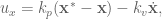
where 


If you define your operational space control signal like this, and then translate this signal into joint torques (using, for example, methods discussed in other posts), you’re going to see a very non-straight trajectory emerge in larger movements as a result of “actuator saturation, and bandwidth and velocity limitations”. In the example of a standard robot, you might run into issues with your motors not being able to actually generate the torques that have been specified, the frequency of control and feedback might not be sufficient, and you could hit hard constraints on system velocity. The solution to this problem was presented in this 1987 paper by Dr. Oussama Khatib, and is pretty slick and very useful, so I thought I’d write it up here for any other unfortunate souls wandering around in ignorance. First though, here’s what it looks like to move large point to point distances without velocity limiting:


As you can see, the system isn’t moving in a straight line, which can be very aggravating if you’ve worked and reworked out the equations and double checked all your parameters, etc etc. A few things, first, when working with simulations it’s easy to forget how ridiculously fast this actually would be in real-time. Even though it takes a minute to simulate the above movement, in real-time, is happening over the course of 200ms. Taking that into account, this is pretty good. Also, there’s an obvious solution here, slow down your movement. The source of this problem is largely that all of the motors are not able to apply the torques specified and move at the required speed. Some of the motors have a lot less mass to throw around and will be able to move at the specified torques, but not all. Hence the not straight trajectory.
You can of course drop the gains on your PD signal, but that’s not really a great methodical solution. So, what can we do?
Well, if we rearrange the PD control signal specified above into

where 

When things are in this form, it becomes a bit more clear what we have to do: limit the desired velocity to be at most some specified maximum velocity of the end-effector, 
Taking 

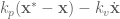
where 


where 


As a result of using this saturation function, the control signal behaves differently depending on whether or not 
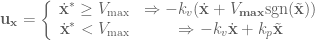
where 


So now the control signal is behaving exactly as desired! Moves the system towards the target, but no faster than the specified maximum velocity. Now our trajectories look like this:


So those are starting to look a lot better! The first thing you’ll notice is that this is a fair bit slower of a movement. Well, actually, it’s waaaayyyy slower because the playback speed here is 4x faster than in that first animation, and this is a movement over 2s. Which has pros and cons, con: it’s slower, pro: it’s straighter, and you’re less likely to be murdered by it. When you move from simulations to real systems that latter point really moves way up the priority list.
Second thing to notice, the system seems to be minimising the error along one dimension, and then along the next, and then arrives at the target. What’s going on? Because the error along each of the 
It’s a liiiiittle bit more complicated than that, but not much. First, we’ll calculate the values being passed in to the saturation function for each
# implement velocity limiting
lamb = kp / kv
x_tilde = xyz - target_xyz
sat = vmax / (lamb * np.abs(x_tilde))
scale = np.ones(3)
if np.any(sat < 1):
    index = np.argmin(sat)
    unclipped = kp * x_tilde[index]
    clipped = kv * vmax * np.sign(x_tilde[index])
    scale = np.ones(3) * clipped / unclipped
    scale[index] = 1
u_xyz = -kv * (dx + np.clip(sat / scale, 0, 1) *
               scale * lamb * x_tilde)
And now, finally, we start getting the trajectories that we’ve been wanting the whole time:


And finally we can rest easy, knowing that our robot is moving at a reasonable speed along a direct path to its goals. Wherever you’d like to use this neato ‘ish you should be able to just paste in the above code, define your vmax, kp, and kv values and be good to go!

Great Travis! (I need to develop something comparable for speech articulators) Best Bernd
Hey Travis! I guess there is a small corection in the part :
“Well, if we rearrange the PD control signal specified above into
u_x = k_v (\dot{\textbf{x}}^* – \dot{\textbf{x}}) “
Ah, good catch! Thank you very much, correction made! 🙂
Hi Travis, very nice write-up! 🙂
Currently, I want to implement velocity limiting in joint-space. The issue I am facing is that the unit/magnitude of vmax correlates in some way to the resulting behavior, but the joint velocities that I get as feedback from the robot are always waaay smaller than vmax. What I would expect is that at least the “fastest” joint is very close to vmax. What I did was basically to calculate:
u_xyz = -kv * (dx + np.clip(sat / scale, 0, 1) * scale * lamb * x_tilde)
and then add the joint-space inertia and compensate for gravity and coriolis in joint-space:
u_tau = M * u_xyz + tau_gc
Perhaps I am thinking the wrong way, but since we limit dimension-wise I guessed that the algorithm could be applied to joint-space as well?
Any help would be really appreciated! 🙂
Hi Dennis,
ah, so it looks like you’re missing the Jacobian transpose multiplication, to change u_xyz from end-effector forces into joint torques.
Although you mention you’re looking to do this in joint space, I’m not sure that velocity limiting is exactly what you’re after though, as it’s intended purpose is limiting the end-effector forces so that joint torques that are too large aren’t specified. So if you’re starting out in joint space (i.e. your target is a set of joint angles rather than some end-effector position) then you’re going to want to use another method to limit your forces.
The simplest would just be to clip the joint torques whenever they get to large, but you could also scale them all down by the same amount whenever one goes over the max to keep their torques relative to each other the same. Could you describe your task / goal a bit more?
Thanks for a great write-up. I was wondering if in the python code for velocity filtering, the ‘scale’ is just equal to ‘sat’ and then we set the value of ‘min’ of ‘sat’ to 1. Is there any need for the explicit naming of clipped and unclipped and then calculating the scale using the formula which is essentially equal to ‘sat’ or am I missing something?