I gave a talk last month at the HALO (Harware and Algorithms for Learning On-achip) workshop at ICCAD (the International Conference on Computed Aided Design). It’s goes over the work from our paper that came out in Frontiers in Neurorobotics in October, titled: Nengo and Low-Power AI Hardware for Robust, Embedded Neurorobotics. I’ve put it up on YouTube, and am sharing it here, now! I recommend watching it at 2x speed, as I talk pretty slowly (I’ve been told it’s a good ASMR voice).
studywolf
a blog for things I encounter while coding and researching neuroscience, motor control, and learning
Tag Archives: Nengo
Converting your Keras model into a spiking neural network
Let’s set the scene: You know Keras, you’ve heard about spiking neural networks (SNNs), and you want to see what all the fuss is about. For some reason. Maybe it’s to take advantage of some cool neuromorphic edge AI hardware, maybe you’re into computational modeling of the brain, maybe you’re masochistic and like a challenge, or you just think SNNs are cool. I won’t question your motives as long as you don’t start making jokes about SkyNet.
Welcome! In this post I’m going to walk through using Nengo DL to convert models built using Keras into SNNs. Nengo is neural modeling and runtime software built and maintained by Applied Brain Research. We started it and have been using it in the Computational Neuroscience Research Group for a long time now. Nengo DL lets you build neural networks using the Nengo API, and then run them using TensorFlow. You can run any kind of network you want in Nengo (ANNs, RNNs, CNNs, SNNs, etc), but here I’ll be focusing on SNNs.
There are a lot of little things to watch out for in this process. In this post I’ll work through the steps to convert and debug a simple network that classifies MNIST digits. The goal is to show you how you can start converting your own networks and some ways you can debug it if you encounter issues. Programming networks with temporal dynamics is a pretty unintuitive process and there’s lots of nuance to learn, but hopefully this will help you get started.
You can find an IPython notebook with all the code you need to run everything here up on my GitHub. The code I’ll be showing in this post is incomplete. I’m going to focus on the building, training, and conversion of the network and leave out parts like imports, loading in MNIST data, etc. To actually run this code you should get the IPython notebook, and make sure you have the latest Nengo, Nengo DL, and all the other dependencies installed.
Build your network in Keras and running it using NengoDL
The network is just going to be a convnet layer and then a fully connected layer. We build this in Keras all per uje … ushe … you-j … usual:
input = tf.keras.Input(shape=(28, 28, 1))
conv1 = tf.keras.layers.Conv2D(
    filters=32,
    kernel_size=3,
    activation=tf.nn.relu,
)(input)
flatten = tf.keras.layers.Flatten()(conv1)
dense1 = tf.keras.layers.Dense(units=10)(flatten)

model = tf.keras.Model(inputs=input, outputs=dense1)
Once the model is made we can generate a Nengo network from this by calling the NengoDL Converter. We pass the converted network into the Simulator, compile with the standard one-hot classification loss function, and start training.
converter = nengo_dl.Converter(
    model,
    swap_activations={tf.nn.relu: nengo.RectifiedLinear()},
)
net = converter.net
nengo_input = converter.inputs[input]
nengo_output = converter.outputs[dense1]

# run training
with nengo_dl.Simulator(net, seed=0) as sim:
    sim.compile(
        optimizer=tf.optimizers.RMSprop(0.001),
        loss={nengo_output: tf.losses.SparseCategoricalCrossentropy(from_logits=True)},
    )

    sim.fit(train_images, {nengo_output: train_labels}, epochs=10)

    # save the parameters to file
    sim.save_params("mnist_params")
In the Converter call you’ll see that there’s a swap_activations keyword. This is for us to map the TensorFlow activation functions to Nengo activation functions. In this case we’re just mapping ReLU to ReLU. After the training is done, we save the trained parameters to file.
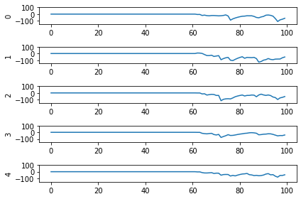
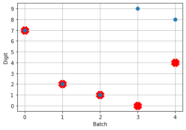
Next, we can load our trained parameters, call the sim.predict function and plot the results:
n_test = 5
with nengo_dl.Simulator(net, seed=0) as sim:
sim.load_params(params_file)
data = sim.predict({nengo_input: test_images[:n_test]})
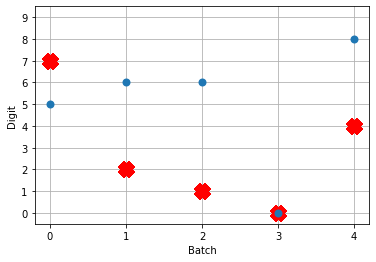
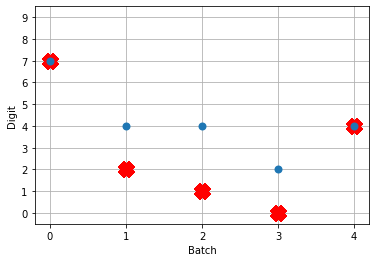
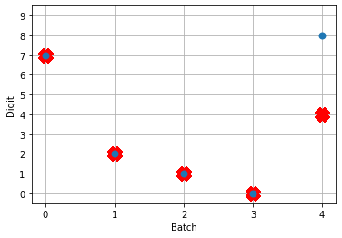
# plot the answer in a big red x
plt.plot(test_labels[:n_test].squeeze(), 'rx', mew=15)
# data[nengo_output].shape = (images, timesteps, n_outputs)
# plot predicted digit from network output on the last time step
plt.plot(np.argmax(data[nengo_output][:, -1], axis=1), 'o', mew=2)

NengoDL inherently accounts for time in its simulations and so the data all needs to be formatted as (n_batches, n_timesteps, n_inputs). In this case everything is using standard rate mode neurons with no internal states that change over time, so simulating the network over time will generate the same output at every time step. When we move to spiking neurons, however, effects of temporal dynamics will be visible.
Convert to spiking neurons
To convert our network to spiking neurons, all we have to do is change the neuron activation function that we map to in the converter when we’re generating the net:
converter = nengo_dl.Converter(
    model,
    swap_activations={tf.nn.relu: nengo.SpikingRectifiedLinear()},
)
net = converter.net
nengo_input = converter.inputs[input]
nengo_output = converter.outputs[dense1]

with nengo_dl.Simulator(net) as sim:
    sim.load_params("mnist_params")
    data = sim.predict({nengo_input: test_images[:n_test]})
So the process is that we create the model using Keras once. Then we can use a NengoDL Converter to create a Nengo network that can be simulated and trained. We save the parameters after training, and now we can use another Converter to create another instance of the network that uses SpikingRectifiedLinear neurons as the activation function. We can then load in the trained parameters that we got from simulating the standard RectifiedLinear rate mode activation function.
The reason that we don’t do the training with the SpikingRectifiedLinear activation function is because of its discontinuities, which cause errors when trying to calculate the derivative in backprop.
So! What kind of results do we get now that we’ve converted into spiking neurons?

Not great! Why is this happening? Good question. It seems like what’s happening is the network is really convinced everything is 5. To investigate, we’re going to need to look at the neural activity.
Plotting the neural activity over time
To be able to see the activity of the neurons, we’re going to need 1) a reference to the ensemble of neurons we’re interested in monitoring, and 2) a Probe to track the activity of those neurons during simulation. This involves changing the network, so we’ll create another converted network and modify it before passing it into our Simulator.
converter = nengo_dl.Converter(
    model,
    swap_activations={tf.nn.relu: nengo.SpikingRectifiedLinear()},
)
net = converter.net

nengo_input = converter.inputs[input]
nengo_output = converter.outputs[dense1]
# get a reference for the neurons that we want to probe
nengo_conv1 = converter.layers[conv1]

# add probe to the network to track the activity of those neurons!
with converter.net as net:
    probe_conv1 = nengo.Probe(nengo_conv1, label='probe_conv1')

with nengo_dl.Simulator(net) as sim:
    sim.load_params("mnist_params")
    data = sim.predict({nengo_input: test_images[:n_test]})
We can use Nengo’s handy rasterplot helper function to plot the activity of the first 3000 neurons:
from nengo.utils.matplotlib import rasterplot
# plot results neural activity from the first n_neurons on the
# first batch (each image is a batch), all time steps
rasterplot(np.arange(n_timesteps), data[probe_conv1][0, :, :n_neurons])
If you have a keen eye and familiar with raster plots, you may notice that there are no spikes. Not a single one! So our network isn’t predicting a 5 for each input, it’s not predicting anything. We’re just getting 5 as output from a learned bias term. Bummer.
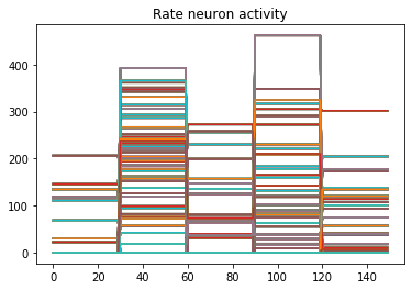
Let’s go back and see what kind of output our rate mode neurons are giving us, maybe that can help explain what’s going on. We can’t use a raster plot, because there are no spikes, but we can use a regular plot.
converter = nengo_dl.Converter(
    model,
    swap_activations={tf.nn.relu: nengo.RectifiedLinear()},
)
net = converter.net

nengo_input = converter.inputs[input]
nengo_output = converter.outputs[dense1]
nengo_conv1 = converter.layers[conv1]

with net:
    probe_conv1 = nengo.Probe(nengo_conv1)

with nengo_dl.Simulator(net) as sim:
    sim.load_params("mnist_params")
    data = sim.predict({nengo_input: test_images[:n_test]})

n_neurons = 5000
print('Max value: ', np.max(data[probe_conv1].flatten()))
# plot activity of first 5000 neurons, all inputs, all time steps
# we reshape the data so it's (n_batches * n_timesteps, n_neurons)
# for ease of plotting
plt.plot(data[probe_conv1][:, :, :n_neurons].reshape(-1, n_neurons))
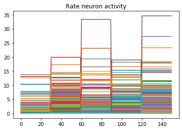
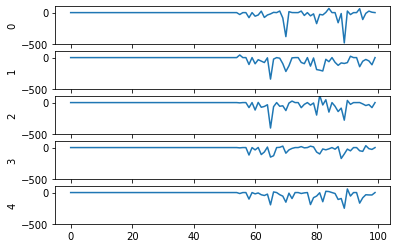
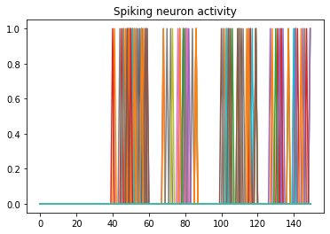
Looking at the rate mode activity of the neurons, we see that the max firing rate is 34.6Hz. That’s about 1 spike every 30 milliseconds. Through an unlucky coincidence we’ve set each image to be presented to the network for 30ms. What could be happening is that neurons are building up to the point of spiking, but the input is switched before they actually spike. To test this, let’s change the number of time steps each image is presented to 100ms, and rerun our spiking simulator.
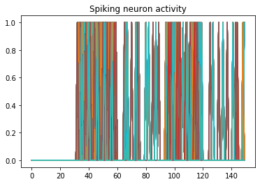
We’ll also switch over to plotting spiking activity the same way as the rate neurons for consistency (and because it’s easier to see if neurons are spiking or not when there’s really sparse activity). One thing you may note below is that I’m plotting activity * dt, instead of just activity like in the rate neuron case. Whenever there’s a spike in Nengo, it’s recorded as 1/dt so that it integrates to 1. Multiplying the probe output by dt means that we see a 1 when there’s one spike per time step, a 2 when there’s two spikes per time step, etc. It just makes it a bit easier to read.
print('Max value: ', np.max(data[probe_conv1].flatten() * dt))
print(data[probe_conv1][:,:,:n_neurons].shape)
plt.plot(data[probe_conv1][:, :, :n_neurons].reshape(-1, n_neurons) * dt)
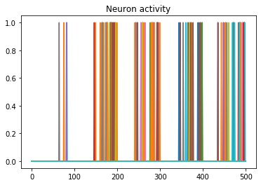
Looking at this plot, we can see a few things. First, whenever an image is presented, there’s a startup period where no spikes occur. Ideally our network will give us some output without having to present input for 50 time steps (the rate network gives us output after 1 time step!) We can address this by increasing the firing rates of the neurons in our network. We’ll come back to this.
Second, even now that we’re getting spikes, the predictions for each image are very poor. Why is that happening? Let’s look at the network output over time when we feed in the first test image:
From this plot it looks like there’s not a clear prediction so much as a bunch of noise. One factor that can contribute to this is that the way things are set up right now, when a neuron spikes that information is only processed by the receiving side for 1 time step. Anthropomorphizing our network, you can think of the output layer as receiving input along the lines of “nothing … nothing … nothing … IT’S A 5! … maybe a 2? … maybe a 3? … IT’S A 5! ..” etc.
It would be useful for us to do a bit of averaging over time. Enter: synapses!
Using synapses to smooth the output of a spiking network
Synapses can come in many forms. The default form in Nengo is a low-pass filter. What this does for us is let the post-synaptic neuron (i.e. the neuron that we’re sending information to) do a bit of integration of the information that is being sent to it. So in the above example the output layer would be receiving input like “nothing … nothing … nothing … looking like a 5 … IT’S A 5! … it’s a 5! … it’s probably a 5 but maybe also a 2 or 3 … IT’S A 5! … ” etc.
Likely it will be more useful for understanding to see the actual network output over time with different low-pass filters applied rather than reading strained metaphors.
To make apply a low-pass filter synapse to all of the connections in our network is easy enough, we just add another modification to the network before passing it into the Simulator:
converter = nengo_dl.Converter(
    model,
    swap_activations={tf.nn.relu: nengo.SpikingRectifiedLinear()},
)
net = converter.net

nengo_input = converter.inputs[input]
nengo_output = converter.outputs[dense1]
nengo_conv1 = converter.layers[conv1]

with net:
    probe_conv1 = nengo.Probe(nengo_conv1)

# set a low-pass filter value on all synapses in the network
for conn in net.all_connections:
    conn.synapse = 0.001

with nengo_dl.Simulator(net) as sim:
    sim.load_params("mnist_params")
    data = sim.predict({nengo_input: test_images[:n_test]})
And here are the results we get for different low-pass filter time constants:
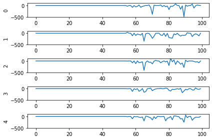


As the time constant on the low-pass filter increases, we can see the output of the network starts smoothing out. It’s important to recognize that there are a few things going on though when we filter values on all of the synapses of the network. The first is that we’re no longer sending sharp spikes between layers, we’re now passing along filtered spikes. The larger the time constant on the filter, the more spread out and smoother the signal will be.
As a result of this: If sending a spike from neuron A to neuron B used to cause neuron B to spike immediately when there was no synaptic filter, that may no longer be the case. It may now take several spikes from neuron A, all close together in time, for neuron B to now spike.
Another thing we want to consider is that we’ve applied a synaptic filter at every layer, so the dynamics of the entire network have changed. Very often you’ll want to be more surgical with the synapses you create, leaving some connections with no synapse and some with large filters to get the best performance out of your network. Currently the way to do this is to print out net.all_connections, find the connections of interest, and then index in specific values. When we print out net.all_connections for this network, we get:
[<Connection at 0x7fd8ac65e4a8 from <Node "conv2d.0.bias"> to <Node (unlabeled) at 0x7fd8ac65ee48>>,
<Connection at 0x7fd969a06b70 from <Node (unlabeled) at 0x7fd8ac65ee48> to <Neurons of <Ensemble "conv2d.0">>>,
<Connection at 0x7fd969a06390 from <Node "input_1"> to <Neurons of <Ensemble "conv2d.0">>>,
<Connection at 0x7fd8afc41470 from <Node "dense.0.bias"> to <Node "dense.0">>,
<Connection at 0x7fd8afc41588 from <Neurons of <Ensemble "conv2d.0">> to <Node "dense.0">>]
The connections of interest for us are from input_1 to conv2d.0, and from conv2d.0 to dense.0. These are the connections the input signals for the network are flowing through, the rest of the connections are just to send in trained bias values to each layer. We can set the synapse value for these connections specifically with the following:
synapses = [None, None, 0.001, None, 0.001]
for conn, synapse in zip(net.all_connections, synapses):
    conn.synapse = synapse
In this case, with just some playing around with different values I wasn’t able to find any synapse values that got better performance than 4/5. But in general being able to set specific synapse values in a spiking neural network is important and you should be aware of how to do it to get the best performance out of your network.
So setting the synapses is able to improve the performance of the network. We’re still taking 100ms to generate output though, and only getting 4/5 of the test set correct. Let’s go back now to the first issue we identified and look at increasing the firing rates of the neurons.
Increasing the firing rates of neurons in the network
There are a few ways to go about this. The first is a somewhat cheeky method that works best for rectified linear (ReLU) neurons, and the second is a more general method that adjusts how training is performed.
Scaling ReLU firing rates
Because we’re using rectified linear neurons in this model, one trick that we can use to increase the firing rates without affecting the functionality of the network is by using a scaling term to multiply the input and divide the output of each neuron. This scaling can work because the rectified linear neuron model is linear in its activation function.
The result of this scaling is more frequent spiking at a lower amplitude. We can implement this using the Nengo DL Converter with the scale_firing_rates keyword:
converter = nengo_dl.Converter(
    model,
    swap_activations={tf.nn.relu: nengo.SpikingRectifiedLinear()},
    scale_firing_rates=gain_scale,
)
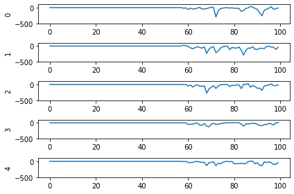
Let’s look at the network output and neural activity plots for gain_scale values of [5, 20, 50].


One thing that’s apparent is as the firing rates go up, the performance of the network gets better. You may notice that for the first image (first 30 time steps) in the spiking activity plots there’s no response. Don’t read too much into that; I’m plotting a random subset of neurons and it just happens that none of them respond to the first image. If I was to plot the activity of all of the neurons we’d see spikes everywhere.
You may also notice that when gain_scale = 50 we’re even getting some neurons that are spiking 2 times per time step. That will happen when the input to the neuron causes the internal state to jump up to twice the threshold for spiking for that neuron. This is not unexpected behaviour.
Using this scale_firing_rates keyword in the Converter is one way to get the performance of our coverted spiking networks to match the performance of rate neuron networks. However, it mainly a trick useful for us for ReLUs (and any other linear activation functions). It would behoove us to figure out another method that will work as well for nonlinear activation functions as well.
Adding a firing rate term to the cost function during training
Let’s go back to the training the network step. Another way to bring the firing rates up is by adding a term to the cost function that will penalize any firing rates outside of some desired range. There are a ton of ways to go about this with different kinds of cost functions. I’m just going to present one cost function term that works for this situation and note that you can build this cost function a whole bunch of different ways. Here’s one:
def put_in_range(x, y, weight=100.0, min=200, max=300):
    index_greater = (y > max)  # find neurons firing faster
    index_lesser = (y < min)  # find neurons firing slower
    error = tf.reduce_sum(y[index_greater] - max) + tf.reduce_sum(min - y[index_lesser])
    return weight * error
The weight parameter lets us set the relative importance of the firing rates cost function term relative to the classification accuracy cost function term. To use this term we need to make a couple of adjustments to our code for training the network:
converter = nengo_dl.Converter(
    model,
    swap_activations={tf.nn.relu: nengo.RectifiedLinear()},
)
net = converter.net

nengo_input = converter.inputs[input]
nengo_output = converter.outputs[dense1]

nengo_conv1 = converter.layers[conv1]
with converter.net as net:
    probe_conv1 = nengo.Probe(nengo_conv1, label='probe_conv1')

# run training
with nengo_dl.Simulator(net) as sim:
    sim.compile(
        optimizer=tf.optimizers.RMSprop(0.001),
        loss={
            nengo_output: tf.losses.SparseCategoricalCrossentropy(from_logits=True),
            probe_conv1: put_in_range,
        }
    )
    sim.fit(
        train_images,
        {nengo_output: train_labels,
         probe_conv1: np.zeros(train_labels.shape)},
        epochs=10)
Mainly what’s been added in this code is our new loss function put_in_range and in the sim.compile call we added probe_conv1: put_in_range to the loss dictionary. This tells Nengo DL to use the put_in_range cost function on the output from probe_conv1, which will be the firing rates of the convolutional layer of neurons in the network.
We also had to add in probe_conv1: np.zeros(train_labels.shape) to the input dictionary in the sim.fit function call. The array specified here is used as the x input to the put_in_range cost function, but since we defined the put_in_range function to be fully determined based only on y (which is the output from probe_conv1) it doesn’t matter what values we pass in there. So I pass in an array of zeros.
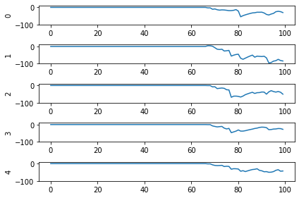
Now when we run the training and prediction in rate mode, the output we get looks like

And we can see that we’re still getting the same performance, but now the firing rates of the neurons are much higher. Let’s see what happens when we convert to spiking neurons now!

Hey, that’s looking much better! This of course is only looking at 5 test images and you’ll want to go through and calculate proper performance statistics using a full test set, but it’s a good start.
Conclusions
This post has looked at how to take a model that you built in Keras and convert it over to a spiking neural network using Nengo DL’s Converter function. This was a simple model, but hopefully it gets across that the conversion to spikes can be an iterative process, and you now have a better sense of some of the steps that you can take to investigate and debug spiking neural network behaviour! In general when tuning your network you’ll use a mix of the different methods we’ve gone through here, depending on the exact situation.
Again a reminder that all of the code for this can be found up on my GitHub.
Also! It’s very much worth checking out the Nengo DL documentation and other examples that they have there. There’s a great introduction for users coming from TensorFlow over to Nengo, and other examples showing how you can integrate non-spiking networks with spiking networks, as well as other ways to optimizing your spiking neural networks. If you start playing around with Nengo and have more questions, please feel free to ask in comments below or even better go to the Nengo forums!
Building a spiking neural model of adaptive arm control
About a year ago I published the work from my thesis in a paper called ‘A spiking neural model of adaptive arm control’. In this paper I presented the Recurrent Error-driven Adaptive Control Hierarchy (REACH) model. The goal of the model is to begin working towards reproducing behavioural level phenomena of human movement with biologically plausible spiking neural networks.
To do this, I start by using three methods from control literature (operational space control, dynamic movement primitives, and non-linear adaptive control) to create an algorithms level model of the motor control system that captures behavioural level phenomena of human movement. Then I explore how this functionality could be mapped to the primate brain and implemented in spiking neurons. Finally, I look at the data generated by this model on the behavioural level (e.g. kinematics of movement), the systems level (i.e. analysis of populations of neurons), and the single-cell level (e.g. correlating neural activity with movement parameters) and compare/contrast with experimental data.
By having a full model framework (from observable behaviour to neural spikes) is to have a more constrained computational model of the motor control system; adding lower-level biological constraints to behavioural models and higher-level behavioural constraints to neural models.
In general, once you have a model, the critical next step is to generating testable predictions that can be used to discriminate between other models with different implementations or underlying algorithms. Discriminative predictions allow us to design experiments that can gather evidence in favour or against different hypotheses of brain function, and provide clues to useful directions for further research. Which is the real contribution of computational modeling.
So that’s a quick overview of the paper; there are quite a few pages of supplementary information that describe the details of the model implementation, and I provided the code and data used to generate the data analysis figures. However, code to explicitly run the model on your own has been missing. As one of the major points of this blog is to provide code for furthering research, this is pretty embarrassing. So, to begin to remedy this, in this post I’m going to work through a REACH framework for building models to control a two-link arm through reaching in a line, tracing a circle, performing the centre-out reaching task, and adapting online to unexpected perturbations during reaching imposed by a joint-velocity based forcefield.
This post is directed towards those who have already read the paper (although not necessarily the supplementary material). To run the scripts you’ll need Nengo, Nengo GUI, and NengoLib all installed. There’s a description of the theory behind the Neural Engineering Framework, which I use extensively in my Nengo modeling, in the paper. I’m hoping that between that and code readability / my explanations below that most will be comfortable starting to play around with the code. But if you’re not, and would like more resources, you can check out the Getting Started page on the Nengo website, the tutorials from How To Build a Brain, and the examples in the Nengo GUI.
You can find all of the code up on my GitHub.
NOTE: I’m using the two-link arm (which is fully implemented in Python) instead of the three-link arm (which has compile issues for Macs) both so that everyone should be able to run the model arm code and to reduce the number of neurons that are required for control, so that hopefully you can run this on you laptop in the event that you don’t have a super power Ubuntu work station. Scaling this model up to the three-link arm is straight-forward though, and I will work on getting code up (for the three-link arm for non-Mac users) as a next project.
Implementing PMC – the trajectory generation system
I’ve talked at length about dynamic movement primitives (DMPs) in previous posts, so I won’t describe those again here. Instead I will focus on their implementation in neurons.
def generate(y_des, speed=1, alpha=1000.0):
    beta = alpha / 4.0

    # generate the forcing function
    forces, _, goals = forcing_functions.generate(
        y_des=y_des, rhythmic=False, alpha=alpha, beta=beta)

    # create alpha synapse, which has point attractor dynamics
    tau = np.sqrt(1.0 / (alpha*beta))
    alpha_synapse = nengolib.Alpha(tau)

    net = nengo.Network('PMC')
    with net:
        net.output = nengo.Node(size_in=2)

        # create a start / stop movement signal
        time_func = lambda t: min(max(
            (t * speed) % 4.5 - 2.5, -1), 1)

        def goal_func(t):
            t = time_func(t)
            if t <= -1:
                return goals[0]
            return goals[1]
        net.goal = nengo.Node(output=goal_func, label='goal')

        # -------------------- Ramp ---------------------------
        ramp_node = nengo.Node(output=time_func, label='ramp')
        net.ramp = nengo.Ensemble(
            n_neurons=500, dimensions=1, label='ramp ens')
        nengo.Connection(ramp_node, net.ramp)

        # ------------------- Forcing Functions ---------------
        def relay_func(t, x):
            t = time_func(t)
            if t <= -1:
                return [0, 0]
            return x
        # the relay prevents forces from being sent on reset
        relay = nengo.Node(output=relay_func, size_in=2)

        domain = np.linspace(-1, 1, len(forces[0]))
        x_func = interpolate.interp1d(domain, forces[0])
        y_func = interpolate.interp1d(domain, forces[1])
        transform=1.0/alpha/beta
        nengo.Connection(net.ramp, relay[0], transform=transform,
                         function=x_func, synapse=alpha_synapse)
        nengo.Connection(net.ramp, relay[1], transform=transform,
                         function=y_func, synapse=alpha_synapse)
        nengo.Connection(relay, net.output)

        nengo.Connection(net.goal[0], net.output[0],
                         synapse=alpha_synapse)
        nengo.Connection(net.goal[1], net.output[1],
                         synapse=alpha_synapse)
    return net
The generate method for the PMC takes in a desired trajectory, y_des, as a parameter. The first thing we do (on lines 5-6) is calculate the forcing function that will push the DMP point attractor along the desired trajectory.
The next thing (on lines 9-10) is creating an Alpha (second-order low-pass filter) synapse. By writing out the dynamics of a point attractor in Laplace space, one of the lab members, Aaron Voelker, noticed that the dynamics could be fully implemented by creating an Alpha synapse with an appropriate choice of tau. I walk through all of the math behind this in this post. Here we’ll use that more compact method and project directly to the output node, which improves performance and reduces the number of neurons.
Inside the PMC network we create a time_func node, which is the pace-setter during simulation. It will output a linear ramp from -1 to 1 every few seconds, with the pace set by the speed parameter, and then pause before restarting.
We also have a goal node, which will provide a target starting and ending point for the trajectory. Both the time_func and goal nodes are created and used as a model simulation convenience, and proposed to be generated elsewhere in the brain (the basal ganglia, why not? #igotreasons #provemewrong).
The ramp ensemble is the most important component of the trajectory generation system. It takes the output from the time_func node as input, and generates the forcing function which will guide our little system through the trajectory that was passed in. The ensemble itself is nothing special, but rather the function that it approximates on its outgoing connection. We set up this function approximation with the following code:
        domain = np.linspace(-1, 1, len(forces[0]))
        x_func = interpolate.interp1d(domain, forces[0])
        y_func = interpolate.interp1d(domain, forces[1])
        transform=1.0/alpha/beta
        nengo.Connection(net.ramp, relay[0], transform=transform,
                         function=x_func, synapse=alpha_synapse)
        nengo.Connection(net.ramp, relay[1], transform=transform,
                         function=y_func, synapse=alpha_synapse)
        nengo.Connection(relay, net.output)
We want the forcing function be generated as the signals represented in the ramp ensemble moves from -1 to 1. To achieve this, we create interpolation functions, x_func and y_func, which are set up to generate the forcing function values mapped to input values between -1 and 1. We pass these functions into the outgoing connections from the ramp population (one for x and one for y). So now when the ramp ensemble is representing -1, 0, and 1 the output along the two connections will be the starting, middle, and ending x and y points of the forcing function trajectory. The transform and synapse are set on each connection with the appropriate gain values and Alpha synapse, respectively, to implement point attractor dynamics.
NOTE: The above DMP implementation can generate a trajectory signal with as many dimensions as you would like, and all that’s required is adding another outgoing Connection projecting from the ramp ensemble.
The last thing in the code is hooking up the goal node to the output, which completes the point attractor implementation.
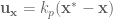
Implementing M1 – the kinematics of operational space control
In REACH, we’ve modelled the primary motor cortex (M1) as responsible for taking in a desired hand movement (i.e. target_position - current_hand_position) and calculating a set of joint torques to carry that out. Explicitly, M1 generates the kinematics component of an OSC signal:

In the paper I did this using several populations of neurons, one to calculate the Jacobian, and then an EnsembleArray to perform the multiplication for the dot product of each dimension separately. Since then I’ve had the chance to rework things and it’s now done entirely in one ensemble.
Now, the set up for the M1 model that computes the above function is to have a single ensemble of neurons that takes in the joint angles, 
Let’s look at the code (where I’ve stripped out the comments and some debugging code):
def generate(arm, kp=1, operational_space=True,
             inertia_compensation=True, means=None, scales=None):

    dim = arm.DOF + 2

    means = np.zeros(dim) if means is None else means
    scales = np.ones(dim) if scales is None else scales
    scale_down, scale_up = generate_scaling_functions(
        np.asarray(means), np.asarray(scales))

    net = nengo.Network('M1')
    with net:
        # create / connect up M1 ------------------------------
        net.M1 = nengo.Ensemble(
            n_neurons=1000, dimensions=dim,
            radius=np.sqrt(dim),
            intercepts=AreaIntercepts(
                dimensions=dim,
                base=nengo.dists.Uniform(-1, .1)))

        # expecting input in form [q, x_des]
        net.input = nengo.Node(output=scale_down, size_in=dim)
        net.output = nengo.Node(size_in=arm.DOF)

        def M1_func(x, operational_space, inertia_compensation):
            """ calculate the kinematics of the OSC signal """
            x = scale_up(x)
            q = x[:arm.DOF]
            x_des = kp * x[arm.DOF:]

            # calculate hand (dx, dy)
            if operational_space:
                J = arm.J(q=q)

                if inertia_compensation:
                    # account for inertia
                    Mx = arm.Mx(q=q)
                    x_des = np.dot(Mx, x_des)
                # transform to joint torques
                u = np.dot(J.T, x_des)
            else:
                u = x_des

                if inertia_compensation:
                    # account for mass
                    M = arm.M(q=q)
                    u = np.dot(M, x_des)

            return u

        # send in system feedback and target information
        # don't account for synapses twice
        nengo.Connection(net.input, net.M1, synapse=None)
        nengo.Connection(
            net.M1, net.output,
            function=lambda x: M1_func(
                x, operational_space, inertia_compensation),
            synapse=None)

    return net
The ensemble of neurons itself is created with a few interesting parameters:
        net.M1 = nengo.Ensemble(
            n_neurons=1000, dimensions=dim,
            radius=np.sqrt(dim),
            intercepts=AreaIntercepts(
                dimensions=dim, base=nengo.dists.Uniform(-1, .1)))
Specifically, the radius and intercepts parameters.
Setting the intercepts
First we’ll discuss setting the intercepts using the AreaIntercepts distribution. The intercepts of a neuron determine how much of state space a neuron is active in, which we’ll refer to as the ‘active proportion’. If you don’t know what kind of functions you want to approximate with your neurons, then you having the active proportions for your ensemble chosen from a uniform distribution is a good starting point. This means that you’ll have roughly the same number of neurons active across all of state space as you do neurons that are active over half of state space as you do neurons that are active over very small portions of state space.
By default, Nengo sets the intercepts such that the distribution of active proportions is uniform for lower dimensional spaces. But when you start moving into higher dimensional spaces (into a hypersphere) the default method breaks down and you get mostly neurons that are either active for all of state space or almost none of state space. The AreaIntercepts class calculates how the intercepts should be set to achieve the desire active proportion inside a hypersphere. There are a lot more details here that you can read up on in this IPython notebook by Dr. Terrence C. Stewart.
What you need to know right now is that we’re setting the intercepts of the neurons such that the percentage of state space for which any given neuron is active is chosen from a uniform distribution between 0% and 55%. In other words, a neuron will maximally be active in 55% of state space, no more. This will let us model more nonlinear functions (such as the kinematics of the OSC signal) with fewer neurons. If this description is clear as mud, I really recommend checking out the IPython notebook linked above to get an intuition for what I’m talking about.
Scaling the input signal
The other parameter we set on the M1 ensemble is the radius. The radius scales the range of input values that the ensemble can represent, which is by default anything inside the unit hypersphere (i.e. hypersphere with radius=1). If the radius is left at this default value, the neural activity will saturate for vectors with magnitude greater than 1, leading to inaccurate vector representation and function approximation for input vectors with magnitude > 1. For lower dimensions this isn’t a terrible problem, but as the dimensions of the state space you’re representing grow it becomes more common for input vectors to have a norm greater than 1. Typically, we’d like to be able to, at a minimum, represent vectors with any number of dimensions where any element can be anywhere between -1 and 1. To do this, all we have to do is calculate the norm of the unit vector size dim, which is np.sqrt(dim) (the magnitude of a vector size dim with all elements set to one).
Now that we’re able to represent vectors where the input values are all between -1 and 1, the last part of this sub-network is scaling the input to be between -1 and 1. We use two scaling functions, scale_down and scale_up. The scale_down function subtracts a mean value and scales the input signal to be between -1 and 1. The scale_up function reverts the vector back to it’s original values so that calculations can be carried out normally on the decoding. In choosing mean and scaling values, there are two ways we can set these functions up:
- Set them generally, based on the upper and lower bounds of the input signal. For M1, the input is
where
is the control signal in end-effector space, we know that the joint angles are always in the range 0 to
(because that’s how the arm simulation is programmed), so we can set the
meansandscalesto befor
a mean of zero is reasonable, and we can choose (arbitrarily, empirically, or analytically) the largest task space control signal we want to represent accurately.
- Or, if we know the model will be performing a specific task, we can look at the range of input values encountered during that task and set the
meansandscalesterms appropriately. For the task of reaching in a straight line, the arm moves in a very limited state space and we can set the mean and we can tune these parameter to be very specific:means=[0.6, 2.2, 0, 0], scales=[.25, .25, .25, .25]
The benefit of the second method, although one can argue it’s parameter tuning and makes things less biologically plausible, is that it lets us run simulations with fewer neurons. The first method works for all of state space, given enough neurons, but seeing as we don’t always want to be simulating 100k+ neurons we’re using the second method here. By tuning the scaling functions more specifically we’re able to run our model using 1k neurons (and could probably get away with fewer). It’s important to keep in mind though that if the arm moves outside the expected range the control will become unstable.
Implementing CB – the dynamics of operational space control
The cerebellum (CB) sub-network has two components to it: dynamics compensation and dynamics adaptation. First we’ll discuss the dynamics compensation. By which I mean the 
Much like the calculating the kinematics term of the OSC signal in M1, we can calculate the entire dynamics compensation term using a single ensemble with an appropriate radius, scaled inputs, and well chosen intercepts.
def generate(arm, kv=1, learning_rate=None, learned_weights=None,
             means=None, scales=None):
    dim = arm.DOF * 2

    means = np.zeros(dim) if means is None else means
    scales = np.ones(dim) if scales is None else scales
    scale_down, scale_up = generate_scaling_functions(
        np.asarray(means), np.asarray(scales))

    net = nengo.Network('CB')
    with net:
        # create / connect up CB --------------------------------
        net.CB = nengo.Ensemble(
            n_neurons=1000, dimensions=dim,
            radius=np.sqrt(dim),
            intercepts=AreaIntercepts(
                dimensions=dim,
                base=nengo.dists.Uniform(-1, .1)))
        # expecting input in form [q, dq, u]
        net.input = nengo.Node(output=scale_down,
                               size_in=dim+arm.DOF+2)
        cb_input = nengo.Node(size_in=dim, label='CB input')
        nengo.Connection(net.input[:dim], cb_input)
        # output is [-Mdq, u_adapt]
        net.output = nengo.Node(size_in=arm.DOF*2)

        def CB_func(x):
            """ calculate the dynamic component of OSC signal """
            x = scale_up(x)
            q = x[:arm.DOF]
            dq = x[arm.DOF:arm.DOF*2]

            # calculate inertia matrix
            M = arm.M(q=q)
            return -np.dot(M, kv * dq)
        # connect up the input and output
        nengo.Connection(net.input[:dim], net.CB)
        nengo.Connection(net.CB, net.output[:arm.DOF],
                         function=CB_func, synapse=None)
I don’t think there’s anything noteworthy going on here, most of the relevant details have already been discussed…so we’ll move on to the adaptation!
Implementing CB – non-linear dynamics adaptation
The final part of the model is the non-linear dynamics adaptation, modelled as a separate ensemble in the cerebellar sub-network (a separate ensemble so that it’s more modular, the learning connection could also come off of the other CB population). I work through the details and proof of the learning rule in the paper, so I’m not going to discuss that here. But I will restate the learning rule here:

where 


The adaptive ensemble can be initialized either using saved weights (passed in with the learned_weights paramater) or as all zeros. It is important to note that setting decoders to all zeros means that does not mean having zero neural activity, so learning will not be affected by this initialization.
        # dynamics adaptation------------------------------------
        if learning_rate is not None:
            net.CB_adapt = nengo.Ensemble(
                n_neurons=1000, dimensions=arm.DOF*2,
                radius=np.sqrt(arm.DOF*2),
                # enforce spiking neurons
                neuron_type=nengo.LIF(),
                intercepts=AreaIntercepts(
                    dimensions=arm.DOF,
                    base=nengo.dists.Uniform(-.5, .2)))

            net.learn_encoders = nengo.Connection(
                net.input[:arm.DOF*2], net.CB_adapt,)

            # if no saved weights were passed in start from zero
            weights = (
                learned_weights if learned_weights is not None
                else np.zeros((arm.DOF, net.CB_adapt.n_neurons)))
            net.learn_conn = nengo.Connection(
                # connect directly to arm so that adaptive signal
                # is not included in the training signal
                net.CB_adapt.neurons, net.output[arm.DOF:],
                transform=weights,
                learning_rule_type=nengo.PES(
                    learning_rate=learning_rate),
                synapse=None)

            nengo.Connection(net.input[dim:dim+2],
                             net.learn_conn.learning_rule,
                             transform=-1, synapse=.01)
    return net
We’re able to implement that learning rule using Nengo’s prescribed error-sensitivity (PES) learning on our connection from the adaptive ensemble to the output. With this set up the system will be able to learn to adapt to perturbations that are functions of the input (set here to be ![[\textbf{q}, \dot{\textbf{q}}]](https://s0.wp.com/latex.php?latex=%5B%5Ctextbf%7Bq%7D%2C+%5Cdot%7B%5Ctextbf%7Bq%7D%7D%5D&bg=ffffff&fg=555555&s=0&c=20201002)
The intercepts in this population are set to values I found worked well for adapting to a few different forces, but it’s definitely a parameter to play with in your own scripts if you’re finding that there’s too much or not enough generalization of the decoded function output across the state space.
One other thing to mention is that we need to have a relay node to amalgamate the control signals output from M1 and the dynamics compensation ensemble in the CB. This signal is used to train the adaptive ensemble, and it’s important that the adaptive ensemble’s output is not included in the training signal, or else the system quickly goes off to positive or negative infinity.
Implementing S1 – a placeholder
The last sub-network in the REACH model is a placeholder for a primary sensory cortex (S1) model. This is just a set of ensembles that represents the feedback from the arm and relay it on to the rest of the model.
def generate(arm, direct_mode=False, means=None, scales=None):
    dim = arm.DOF*2 + 2  # represents [q, dq, hand_xy]

    means = np.zeros(dim) if means is None else means
    scales = np.ones(dim) if scales is None else scales
    scale_down, scale_up = generate_scaling_functions(
        np.asarray(means), np.asarray(scales))

    net = nengo.Network('S1')
    with net:
        # create / connect up S1 --------------------------------
        net.S1 = nengo.networks.EnsembleArray(
            n_neurons=50, n_ensembles=dim)

        # expecting input in form [q, x_des]
        net.input = nengo.Node(output=scale_down, size_in=dim)
        net.output = nengo.Node(
            lambda t, x: scale_up(x), size_in=dim)

        # send in system feedback and target information
        # don't account for synapses twice
        nengo.Connection(net.input, net.S1.input, synapse=None)
        nengo.Connection(net.S1.output, net.output, synapse=None)

    return net
Since there’s no function that we’re decoding off of the represented variables we can use separate ensembles to represent each dimension with an EnsembleArray. If we were going to decode some function of, for example, q0 and dq0, then we would need an ensemble that represents both variables. But since we’re just decoding out f(x) = x, using an EnsembleArray is a convenient way to decrease the number of neurons needed to accurately represent the input.
Creating a model using the framework
The REACH model has been set up to be as much of a plug and play system as possible. To generate a model you first create the M1, PMC, CB, and S1 networks, and then they’re all hooked up to each other using the framework.py file. Here’s an example script that controls the arm to trace a circle:
def generate():
    kp = 200
    kv = np.sqrt(kp) * 1.5

    center = np.array([0, 1.25])
    arm_sim = arm.Arm2Link(dt=1e-3)
    # set the initial position of the arm
    arm_sim.init_q = arm_sim.inv_kinematics(center)
    arm_sim.reset()

    net = nengo.Network(seed=0)
    with net:
        net.dim = arm_sim.DOF
        net.arm_node = arm_sim.create_nengo_node()
        net.error = nengo.Ensemble(1000, 2)
        net.xy = nengo.Node(size_in=2)

        # create an M1 model -------------------------------------
        net.M1 = M1.generate(arm_sim, kp=kp,
                             operational_space=True,
                             inertia_compensation=True,
                             means=[0.6, 2.2, 0, 0],
                             scales=[.5, .5, .25, .25])

        # create an S1 model -------------------------------------
        net.S1 = S1.generate(arm_sim,
                             means=[.6, 2.2, -.5, 0, 0, 1.25],
                             scales=[.5, .5, 1.7, 1.5, .75, .75])

        # subtract current position to get task space direction
        nengo.Connection(net.S1.output[net.dim*2:], net.error,
                         transform=-1)

        # create a trajectory for the hand to follow -------------
        x = np.linspace(0.0, 2.0*np.pi, 100)
        PMC_trajectory = np.vstack([np.cos(x) * .5,
                                    np.sin(x) * .5])
        PMC_trajectory += center[:, None]
        # create / connect up PMC --------------------------------
        net.PMC = PMC.generate(PMC_trajectory, speed=1)
        # send target for calculating control signal
        nengo.Connection(net.PMC.output, net.error)
        # send target (x,y) for plotting
        nengo.Connection(net.PMC.output, net.xy)

        net.CB = CB.generate(arm_sim, kv=kv,
                             means=[0.6, 2.2, -.5, 0],
                             scales=[.5, .5, 1.6, 1.5])

    model = framework.generate(net=net, probes_on=True)
    return model
In line 50 you can see the call to the framework code, which will hook up the most common connections that don’t vary between the different scripts.
The REACH model has assigned functionality to each area / sub-network, and you can see the expected input / output in the comments at the top of each sub-network file, but the implementations are open. You can create your own M1, PMC, CB, or S1 sub-networks and try them out in the context of a full model that generates high-level movement behaviour.
Running the model
To run the model you’ll need Nengo, Nengo GUI, and NengoLib all installed. You can then pull open Nengo GUI and load any of the a# scripts. In all of these scripts the S1 model is just an ensemble that represents the output from the arm_node. Here’s what each of the scripts does:
a01has a spiking M1 and CB, dynamics adaptation turned off. The model guides the arm in reaching in a straight line to a single target and back.a02has a spiking M1, PMC, and CB, dynamics adaptation turned off. The PMC generates a path for the hand to follow that traces out a circle.a03has a spiking M1, PMC, and CB, dynamics adaptation turned off. The PMC generates a path for the joints to follow, which moves the hand in a straight line to a target and back.a04has a spiking M1 and CB, dynamics adaptation turned off. The model performs the centre-out reaching task, starting at a central point and reaching to 8 points around a circle.a05has a spiking M1 and CB, and dynamics adaptation turned on. The model performs the centre-out reaching task, starting at a central point and reaching to 8 points around a circle. As the model reaches, a forcefield is applied based on the joint velocities that pushes the arm as it tries to reach the target. After 100-150 seconds of simulation the arm has adapted and learned to reach in a straight line again.
Here’s what it looks like when you pull open a02 in Nengo GUI:

I’m not going to win any awards for arm animation, but! It’s still a useful visualization, and if anyone is proficient in javascript and want’s to improve it, please do! You can see the network architecture in the top left, the spikes generated by M1 and CB to the right of that, the arm in the bottom left, and the path traced out by the hand just to the right of that. On the top right you can see the a02 script code, and below that the Nengo console.
Conclusions
One of the most immediate extensions (aside from any sort of model of S1) that comes to mind here is implementing a more detailed cerebellar model, as there are several anatomically detailed models which have the same supervised learner functionality (for example (Yamazaki and Nagao, 2012)).
Hopefully people find this post and the code useful for their own work, or at least interesting! In the ideal scenario this would be a community project, where researchers add models of different brain areas and we end up with a large library of implementations to build larger models with in a Mr. Potato Head kind of fashion.
You can find all of the code up on my GitHub. And again, this code all should have been publicly available along with the publication. Hopefully the code proves useful! If you have any questions about it please don’t hesitate to make a comment here or contact me through email, and I’ll get back to you as soon as I can.
Improving neural models by compensating for discrete rather than continuous filter dynamics when simulating on digital systems
This is going to be a pretty niche post, but there is some great work by Aaron Voelker from my old lab that has inspired me to do a post. The work is from an upcoming paper, which is all up on Aaron’s GitHub. It applies to building neural models using the Neural Engineering Framework (NEF). There’s a bunch of material on the NEF out there already, (e.g. the book How to Build a Brain by Dr. Chris Eliasmith, an online intro, and you can also check out Nengo, which is neural model development software with some good tutorials on the NEF) so I’m going to assume you already know the basics of the NEF for this post.
Additionally, this is applicable to simulating these models on digital systems, which, probably, most of you are. If you’re not, however! Then use standard NEF methods.
And then last note before starting, these methods are most relevant for systems with fast dynamics (relative to simulation time). If your system dynamics are pretty slow, you can likely get away with the continuous time solution if you resist change and learning. And we’ll see this in the example point attractor system at the end of the post! But even for slowly evolving systems, I would still recommend at least skipping to the end and seeing how to use the library shortcuts when coding your own models. The example code is also all up on my GitHub.
NEF modeling with continuous lowpass filter dynamics
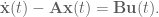
Basic state space equations for linear time-invariant (LTI) systems (i.e. dynamics can be captured with a matrix and the matrices don’t change over time) are:
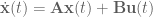
where
is the system state,
is the system output,
is called the input matrix,
is called the output matrix, and
is called the feedthrough matrix,
and the system diagram looks like this:

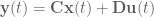
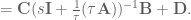
and the transfer function, which is written in Laplace space and captures the system output over system input, for the system is
where 
Now, because it’s a neural system we don’t have a perfect integrator in the middle, we instead have a synaptic filter, 

So our goal is: given some synaptic filter 


Alrighty. Let’s do that.
The transfer function for our neural system is

The effect of the synapse is well captured by a lowpass filter, 


To get this into a form where we can start to modify the system state matrices to compensate for the filter effects, we have to isolate 


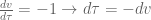
OK. Now, we can make


then we get


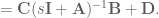
and voila! We have created an 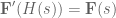
So, to compensate for the continuous lowpass filter, we use 

And so that’s what we’ve been doing for a long time when building our models. Assuming a continuous lowpass filter and going along our merry way. Aaron, however, shrewdly noticed that computers are digital, and thusly that the standard NEF methods are not a fully accurate way of compensating for the filter that is actually being applied in simulation.
To convert our continuous system state equations to discrete state equations we need to make two changes: 1) the first is a variable change to denote the that we’re in discrete time, and we’ll use 

The first step is easy, the second step more complicated. To discretize the system we’ll use the zero-order hold (ZOH) method (also referred to as discretization assuming zero-order hold).
Zero-order hold discretization
Zero-order hold (ZOH) systems simply hold their input over a specified amount of time. The use of ZOH here is that during discretization we assume the input control signal stays constant until the next sample time.
There are good write ups on the derivation of the discretization both on wikipedia and in these course notes from Purdue. I mostly followed the wikipedia derivation, but there were a few steps that get glossed over, so I thought I’d just write it out fully here and hopefully save someone some pain. Also for just a general intro I found these slides from Paul Oh at Drexel University really helpful.
OK. First we’ll solve an LTI system, and then we’ll discretize it.
So, you’ve got yourself a continuous LTI system
and you want to solve for 
Looking through our identity library to find something that might help us here (after a long and grueling search) we come across:
We now left multiply our system by 

Looking at this carefully, we identify the left-hand side as the result of a chain rule, so we can rewrite it as
From here we integrate both sides, giving


To isolate the 


OK! We solved for
To discretize our solution we’re going to assume that we’re sampling the system at even intervals, i.e. each sample is at 


![\textbf{x}[k] = \textbf{x}(kT).](https://s0.wp.com/latex.php?latex=%5Ctextbf%7Bx%7D%5Bk%5D+%3D+%5Ctextbf%7Bx%7D%28kT%29.&bg=ffffff&fg=555555&s=0&c=20201002)
So using our new notation, we have
![\textbf{x}[k] = \textrm{e}^{\textbf{A}kT}\textbf{x}(0) + \textrm{e}^{\textbf{A}kT}\int_0^{kT} \textrm{e}^{-\textbf{A}\tau}\textbf{Bu}(\tau) d\tau.](https://s0.wp.com/latex.php?latex=%5Ctextbf%7Bx%7D%5Bk%5D+%3D+%5Ctextrm%7Be%7D%5E%7B%5Ctextbf%7BA%7DkT%7D%5Ctextbf%7Bx%7D%280%29+%2B+%5Ctextrm%7Be%7D%5E%7B%5Ctextbf%7BA%7DkT%7D%5Cint_0%5E%7BkT%7D+%5Ctextrm%7Be%7D%5E%7B-%5Ctextbf%7BA%7D%5Ctau%7D%5Ctextbf%7BBu%7D%28%5Ctau%29+d%5Ctau.&bg=ffffff&fg=555555&s=0&c=20201002)
Now we want to get things back into the form:
![\textbf{x}[k+1] = \textbf{A}_d\textbf{x}[k] + \textbf{B}_d\textbf{u}[k].](https://s0.wp.com/latex.php?latex=%5Ctextbf%7Bx%7D%5Bk%2B1%5D+%3D+%5Ctextbf%7BA%7D_d%5Ctextbf%7Bx%7D%5Bk%5D+%2B+%5Ctextbf%7BB%7D_d%5Ctextbf%7Bu%7D%5Bk%5D.&bg=ffffff&fg=555555&s=0&c=20201002)
To start, let’s write out the equation for
![\textbf{x}[k + 1]](https://s0.wp.com/latex.php?latex=%5Ctextbf%7Bx%7D%5Bk+%2B+1%5D&bg=ffffff&fg=555555&s=0&c=20201002)
![\textbf{x}[k+1] = \textrm{e}^{\textbf{A}(k+1)T}\textbf{x}(0) + \textrm{e}^{\textbf{A}(k+1)T}\int_0^{(k+1)T} \textrm{e}^{-\textbf{A}\tau}\textbf{Bu}(\tau) d\tau.](https://s0.wp.com/latex.php?latex=%5Ctextbf%7Bx%7D%5Bk%2B1%5D+%3D+%5Ctextrm%7Be%7D%5E%7B%5Ctextbf%7BA%7D%28k%2B1%29T%7D%5Ctextbf%7Bx%7D%280%29+%2B+%5Ctextrm%7Be%7D%5E%7B%5Ctextbf%7BA%7D%28k%2B1%29T%7D%5Cint_0%5E%7B%28k%2B1%29T%7D+%5Ctextrm%7Be%7D%5E%7B-%5Ctextbf%7BA%7D%5Ctau%7D%5Ctextbf%7BBu%7D%28%5Ctau%29+d%5Ctau.&bg=ffffff&fg=555555&s=0&c=20201002)
We want to relate ![\textbf{x}[k+1]](https://s0.wp.com/latex.php?latex=%5Ctextbf%7Bx%7D%5Bk%2B1%5D&bg=ffffff&fg=555555&s=0&c=20201002)
![\textbf{x}[k]](https://s0.wp.com/latex.php?latex=%5Ctextbf%7Bx%7D%5Bk%5D&bg=ffffff&fg=555555&s=0&c=20201002)

![\textrm{e}^{\textbf{A}T}\textbf{x}[k] = \textrm{e}^{\textbf{A}(k+1)T}\textbf{x}(0) + \textrm{e}^{\textbf{A}(k+1)T}\int_0^{kT} \textrm{e}^{-\textbf{A}\tau}\textbf{Bu}(\tau) d\tau,](https://s0.wp.com/latex.php?latex=%5Ctextrm%7Be%7D%5E%7B%5Ctextbf%7BA%7DT%7D%5Ctextbf%7Bx%7D%5Bk%5D+%3D+%5Ctextrm%7Be%7D%5E%7B%5Ctextbf%7BA%7D%28k%2B1%29T%7D%5Ctextbf%7Bx%7D%280%29+%2B+%5Ctextrm%7Be%7D%5E%7B%5Ctextbf%7BA%7D%28k%2B1%29T%7D%5Cint_0%5E%7BkT%7D+%5Ctextrm%7Be%7D%5E%7B-%5Ctextbf%7BA%7D%5Ctau%7D%5Ctextbf%7BBu%7D%28%5Ctau%29+d%5Ctau%2C&bg=ffffff&fg=555555&s=0&c=20201002)
and can rearrange to solve for a term we saw in
![\textrm{e}^{\textbf{A}(k+1)T}\textbf{x}(0) = \textrm{e}^{\textbf{A}T}\textbf{x}[k] - \textrm{e}^{\textbf{A}(k+1)T}\int_0^{kT} \textrm{e}^{-\textbf{A}\tau}\textbf{Bu}(\tau) d\tau.](https://s0.wp.com/latex.php?latex=%5Ctextrm%7Be%7D%5E%7B%5Ctextbf%7BA%7D%28k%2B1%29T%7D%5Ctextbf%7Bx%7D%280%29+%3D+%5Ctextrm%7Be%7D%5E%7B%5Ctextbf%7BA%7DT%7D%5Ctextbf%7Bx%7D%5Bk%5D+-+%5Ctextrm%7Be%7D%5E%7B%5Ctextbf%7BA%7D%28k%2B1%29T%7D%5Cint_0%5E%7BkT%7D+%5Ctextrm%7Be%7D%5E%7B-%5Ctextbf%7BA%7D%5Ctau%7D%5Ctextbf%7BBu%7D%28%5Ctau%29+d%5Ctau.&bg=ffffff&fg=555555&s=0&c=20201002)
Plugging this in, we get
![\textbf{x}[k+1] = \textrm{e}^{\textbf{A}T}\textbf{x}[k] - \textrm{e}^{\textbf{A}(k+1)T}(\int_0^{kT} \textrm{e}^{-\textbf{A}\tau}\textbf{Bu}(\tau) d\tau + \int_0^{(k+1)T} \textrm{e}^{-\textbf{A}\tau}\textbf{Bu}(\tau) d\tau),](https://s0.wp.com/latex.php?latex=%5Ctextbf%7Bx%7D%5Bk%2B1%5D+%3D+%5Ctextrm%7Be%7D%5E%7B%5Ctextbf%7BA%7DT%7D%5Ctextbf%7Bx%7D%5Bk%5D+-+%5Ctextrm%7Be%7D%5E%7B%5Ctextbf%7BA%7D%28k%2B1%29T%7D%28%5Cint_0%5E%7BkT%7D+%5Ctextrm%7Be%7D%5E%7B-%5Ctextbf%7BA%7D%5Ctau%7D%5Ctextbf%7BBu%7D%28%5Ctau%29+d%5Ctau+%2B+%5Cint_0%5E%7B%28k%2B1%29T%7D+%5Ctextrm%7Be%7D%5E%7B-%5Ctextbf%7BA%7D%5Ctau%7D%5Ctextbf%7BBu%7D%28%5Ctau%29+d%5Ctau%29%2C&bg=ffffff&fg=555555&s=0&c=20201002)
![\textbf{x}[k+1] = \textrm{e}^{\textbf{A}T}\textbf{x}[k] - \textrm{e}^{\textbf{A}(k+1)T}\int_{kT}^{(k+1)T} \textrm{e}^{-\textbf{A}\tau}\textbf{Bu}(\tau) d\tau.](https://s0.wp.com/latex.php?latex=%5Ctextbf%7Bx%7D%5Bk%2B1%5D+%3D+%5Ctextrm%7Be%7D%5E%7B%5Ctextbf%7BA%7DT%7D%5Ctextbf%7Bx%7D%5Bk%5D+-+%5Ctextrm%7Be%7D%5E%7B%5Ctextbf%7BA%7D%28k%2B1%29T%7D%5Cint_%7BkT%7D%5E%7B%28k%2B1%29T%7D+%5Ctextrm%7Be%7D%5E%7B-%5Ctextbf%7BA%7D%5Ctau%7D%5Ctextbf%7BBu%7D%28%5Ctau%29+d%5Ctau.&bg=ffffff&fg=555555&s=0&c=20201002)
OK, we’re getting close.
At this point we’ve got things in the right form, but we can still clean up that second term on the right-hand side quite a bit. First, note that using our starting assumption (that 

![\textbf{x}[k+1] = \textrm{e}^{\textbf{A}T}\textbf{x}[k] - \textrm{e}^{\textbf{A}(k+1)T}\int_{kT}^{(k+1)T} \textrm{e}^{-\textbf{A}\tau}d\tau \textbf{Bu}[k].](https://s0.wp.com/latex.php?latex=%5Ctextbf%7Bx%7D%5Bk%2B1%5D+%3D+%5Ctextrm%7Be%7D%5E%7B%5Ctextbf%7BA%7DT%7D%5Ctextbf%7Bx%7D%5Bk%5D+-+%5Ctextrm%7Be%7D%5E%7B%5Ctextbf%7BA%7D%28k%2B1%29T%7D%5Cint_%7BkT%7D%5E%7B%28k%2B1%29T%7D+%5Ctextrm%7Be%7D%5E%7B-%5Ctextbf%7BA%7D%5Ctau%7Dd%5Ctau+%5Ctextbf%7BBu%7D%5Bk%5D.&bg=ffffff&fg=555555&s=0&c=20201002)
Next, bring that 
![\textbf{x}[k+1] = \textrm{e}^{\textbf{A}T}\textbf{x}[k] - \int_{kT}^{(k+1)T} \textrm{e}^{\textbf{A}((k+1)T - \tau)}d\tau \textbf{Bu}[k].](https://s0.wp.com/latex.php?latex=%5Ctextbf%7Bx%7D%5Bk%2B1%5D+%3D+%5Ctextrm%7Be%7D%5E%7B%5Ctextbf%7BA%7DT%7D%5Ctextbf%7Bx%7D%5Bk%5D+-+%5Cint_%7BkT%7D%5E%7B%28k%2B1%29T%7D+%5Ctextrm%7Be%7D%5E%7B%5Ctextbf%7BA%7D%28%28k%2B1%29T+-+%5Ctau%29%7Dd%5Ctau+%5Ctextbf%7BBu%7D%5Bk%5D.&bg=ffffff&fg=555555&s=0&c=20201002)
And now we’re going to simplify the integral using variable substitution. Let 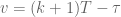


![\textbf{x}[k+1] = \textrm{e}^{\textbf{A}T}\textbf{x}[k] - \int_T^0 \textrm{e}^{\textbf{A}v}dv \textbf{Bu}[k].](https://s0.wp.com/latex.php?latex=%5Ctextbf%7Bx%7D%5Bk%2B1%5D+%3D+%5Ctextrm%7Be%7D%5E%7B%5Ctextbf%7BA%7DT%7D%5Ctextbf%7Bx%7D%5Bk%5D+-+%5Cint_T%5E0+%5Ctextrm%7Be%7D%5E%7B%5Ctextbf%7BA%7Dv%7Ddv+%5Ctextbf%7BBu%7D%5Bk%5D.&bg=ffffff&fg=555555&s=0&c=20201002)
The astute will notice our integral integrates from T to 0 instead of 0 to T. Fortunately for us, we know 

![\textbf{x}[k+1] = \textrm{e}^{\textbf{A}T}\textbf{x}[k] + \int_0^T \textrm{e}^{\textbf{A}v}dv \textbf{Bu}[k].](https://s0.wp.com/latex.php?latex=%5Ctextbf%7Bx%7D%5Bk%2B1%5D+%3D+%5Ctextrm%7Be%7D%5E%7B%5Ctextbf%7BA%7DT%7D%5Ctextbf%7Bx%7D%5Bk%5D+%2B+%5Cint_0%5ET+%5Ctextrm%7Be%7D%5E%7B%5Ctextbf%7BA%7Dv%7Ddv+%5Ctextbf%7BBu%7D%5Bk%5D.&bg=ffffff&fg=555555&s=0&c=20201002)
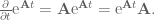
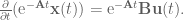
And finally, we can evaluate our integral by recalling that 
![\textbf{x}[k+1] = \textrm{e}^{\textbf{A}T}\textbf{x}[k] + \textbf{A}^{-1} \textrm{e}^{\textbf{A}v}|^T_{v=0} \textbf{Bu}[k].](https://s0.wp.com/latex.php?latex=%5Ctextbf%7Bx%7D%5Bk%2B1%5D+%3D+%5Ctextrm%7Be%7D%5E%7B%5Ctextbf%7BA%7DT%7D%5Ctextbf%7Bx%7D%5Bk%5D+%2B+%5Ctextbf%7BA%7D%5E%7B-1%7D+%5Ctextrm%7Be%7D%5E%7B%5Ctextbf%7BA%7Dv%7D%7C%5ET_%7Bv%3D0%7D+%5Ctextbf%7BBu%7D%5Bk%5D.&bg=ffffff&fg=555555&s=0&c=20201002)
![\textbf{x}[k+1] = \textrm{e}^{\textbf{A}T}\textbf{x}[k] + \textbf{A}^{-1} (\textrm{e}^{\textbf{A}T} - \textrm{e}^0) \textbf{Bu}[k].](https://s0.wp.com/latex.php?latex=%5Ctextbf%7Bx%7D%5Bk%2B1%5D+%3D+%5Ctextrm%7Be%7D%5E%7B%5Ctextbf%7BA%7DT%7D%5Ctextbf%7Bx%7D%5Bk%5D+%2B+%5Ctextbf%7BA%7D%5E%7B-1%7D+%28%5Ctextrm%7Be%7D%5E%7B%5Ctextbf%7BA%7DT%7D+-+%5Ctextrm%7Be%7D%5E0%29+%5Ctextbf%7BBu%7D%5Bk%5D.&bg=ffffff&fg=555555&s=0&c=20201002)
![\textbf{x}[k+1] = \textrm{e}^{\textbf{A}T}\textbf{x}[k] + \textbf{A}^{-1} (\textrm{e}^{\textbf{A}T} - \textbf{I}) \textbf{Bu}[k].](https://s0.wp.com/latex.php?latex=%5Ctextbf%7Bx%7D%5Bk%2B1%5D+%3D+%5Ctextrm%7Be%7D%5E%7B%5Ctextbf%7BA%7DT%7D%5Ctextbf%7Bx%7D%5Bk%5D+%2B+%5Ctextbf%7BA%7D%5E%7B-1%7D+%28%5Ctextrm%7Be%7D%5E%7B%5Ctextbf%7BA%7DT%7D+-+%5Ctextbf%7BI%7D%29+%5Ctextbf%7BBu%7D%5Bk%5D.&bg=ffffff&fg=555555&s=0&c=20201002)
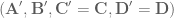
We did it! The state and input matrices for our digital system are:

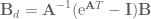
And that’s the hard part of discretization, the rest of the system is easy:
where, fortunately for us


This then gives us our discrete system transfer function:

NEF modeling with continuous lowpass filter dynamics
Now that we know how to discretize our system, we can look at compensating for the lowpass filter dynamics in discrete time. The equation for the discrete time lowpass filter is

where

Plugging that in to the discrete transfer fuction gets us


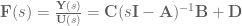
and we see that if we choose
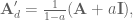

then we get


And now congratulations are in order. Proper compensation for the discrete lowpass filter dynamics has finally been achieved!
Point attractor example
What difference does this actually make in modelling? Well, everyone likes examples, so let’s have one.
Here are the dynamics for a second-order point attractor system:
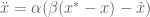
with 


Converting this from a second order system to a first order system we have
![\left [ \begin{array}{c} \dot{x} \\ \ddot{x} \end{array} \right ] = \left [ \begin{array}{cc}0 & 1 \\ -\alpha\beta & -\alpha \end{array} \right] \left [ \begin{array}{c} x \\ \dot{x} \end{array} \right ] + \left [ \begin{array}{c}0 \\ \alpha\beta \end{array} \right] \left [ \begin{array}{c} 0 \\ x^* \end{array} \right ]](https://s0.wp.com/latex.php?latex=%5Cleft+%5B+%5Cbegin%7Barray%7D%7Bc%7D+%5Cdot%7Bx%7D+%5C%5C+%5Cddot%7Bx%7D+%5Cend%7Barray%7D+%5Cright+%5D+%3D+%5Cleft+%5B+%5Cbegin%7Barray%7D%7Bcc%7D0+%26+1+%5C%5C+-%5Calpha%5Cbeta+%26+-%5Calpha+%5Cend%7Barray%7D+%5Cright%5D+%5Cleft+%5B+%5Cbegin%7Barray%7D%7Bc%7D+x+%5C%5C+%5Cdot%7Bx%7D+%5Cend%7Barray%7D+%5Cright+%5D+%2B+%5Cleft+%5B+%5Cbegin%7Barray%7D%7Bc%7D0+%5C%5C+%5Calpha%5Cbeta+%5Cend%7Barray%7D+%5Cright%5D+%5Cleft+%5B+%5Cbegin%7Barray%7D%7Bc%7D+0+%5C%5C+x%5E%2A+%5Cend%7Barray%7D+%5Cright+%5D+&bg=ffffff&fg=555555&s=0&c=20201002)
which we’ll rewrite compactly as

OK, we’ve got our state space equation of the dynamical system we want to implement.
Given a simulation time step 


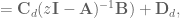
Great! Easy. Now we can calculate the state matrices that will compensate for the discrete lowpass filter:
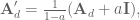

where 
Alright! So that’s our system now, a basic point attractor implementation in Nengo 2.3 looks like this:
tau = 0.1  # synaptic time constant

# the A matrix for our point attractor
A = np.array([[0.0, 1.0],
              [-alpha*beta, -alpha]])

# the B matrix for our point attractor
B = np.array([[0.0], [alpha*beta]])

# account for discrete lowpass filter
a = np.exp(-dt/tau)
if analog:
    A = tau * A + np.eye(2)
    B = tau * B
else:
    # discretize
    Ad = expm(A*dt)
    Bd = np.dot(np.linalg.inv(A), np.dot((Ad - np.eye(2)), B))
    A = 1.0 / (1.0 - a) * (Ad - a * np.eye(2))
    B = 1.0 / (1.0 - a) * Bd

net = nengo.Network(label='Point Attractor')
net.config[nengo.Connection].synapse = nengo.Lowpass(tau)

with config, net:
    net.ydy = nengo.Ensemble(n_neurons=n_neurons, dimensions=2,
        # set it up so neurons are tuned to one dimensions only
        encoders=nengo.dists.Choice([[1, 0], [-1, 0], [0, 1], [0, -1]]))
    # set up Ax part of point attractor
    nengo.Connection(net.ydy, net.ydy, transform=A)

    # hook up input
    net.input = nengo.Node(size_in=1, size_out=1)
    # set up Bu part of point attractor
    nengo.Connection(net.input, net.ydy, transform=B)

    # hook up output
    net.output = nengo.Node(size_in=1, size_out=1)
    # add in forcing function
    nengo.Connection(net.ydy[0], net.output, synapse=None)
Note that for calculating Ad we’re using expm which is the matrix exp function from scipy.linalg package. The numpy.exp does an elementwise exp, which is definitely not what we want here, and you will get some confusing bugs if you’re not careful.
Code for implementing and also testing under some different gains is up on my GitHub, and generates the following plots for dt=0.001:

In the above results you can see that the when the gains are low, and thus the system dynamics are slower, that you can’t really tell a difference between the continuous and discrete filter compensation. But! As you get larger gains and faster dynamics, the resulting effects become much more visible.
If you’re building your own system, then I also recommend using the ss2sim function from Aaron’s nengolib library. It automatically handles compensation for any synapses and generates the matrices that account for discrete or continuous implementations automatically. Using the library looks like:
tau = 0.1  # synaptic time constant
synapse = nengo.Lowpass(tau)

# the A matrix for our point attractor
A = np.array([[0.0, 1.0],
              [-alpha*beta, -alpha]])

# the B matrix for our point attractor
B = np.array([[0.0], [alpha*beta]])

from nengolib.synapses import ss2sim
C = np.eye(2)
D = np.zeros((2, 2))
linsys = ss2sim((A, B, C, D),
                synapse=synapse,
                dt=None if analog else dt)
A = linsys.A
B = linsys.B
Conclusions
So there you are! Go forward and model free of error introduced by improperly accounting for discrete simulation! If, like me, you’re doing anything with neural modelling and motor control (i.e. systems with very quickly evolving dynamics), then hopefully you’ve found all this work particularly interesting, as I did.
There’s a ton of extensions and different directions that this work can be and has already been taken, with a bunch of really neat systems developed using this more accurate accounting for synaptic filtering as a base. You can read up on this and applications to modelling time delays and time cells and lots lots more up on Aaron’s GitHub, and hisrecent papers, which are listed on his lab webpage.
Setting up an arm simulation interface in Nengo 2
I got an email the other day asking about how to set up an arm controller in Nengo, where they had been working from the Spaun code to strip away things until they had just the motor portion left they could play with. I ended up putting together a quick script to get them started and thought I would share it here in case anyone else was interested. It’s kind of fun because it shows off some of the new GUI and node interfacing. Note that you’ll need nengo_gui version .15+ for this to work. In general I recommend getting the dev version installed, as it’s stable and updates are made all the time improving functionality.
Nengo 1.4 core was all written in Java, with Jython and Python scripting thrown in on top, and since then a lot of work has gone into the re-write of the entire code base for Nengo 2. Nengo 2 is now written in Python, all the scripting is in Python, and we have a kickass GUI and support for running neural simulations on CPUs, GPUs, and specialized neuromorphic hardware like SpiNNaKer. I super recommend checking it out if you’re at all interested in neural modelling, we’ve got a bunch of tutorials up and a very active support board to help with any questions or problems. You can find the simulator code for installation here: https://github.com/nengo/nengo and the GUI code here: https://github.com/nengo/nengo_gui, where you can also find installation instructions.
And once you have that up and running, to run an arm simulation you can download and run the following code I have up on my GitHub. When you pop it open at the top is a run_in_GUI boolean, which you can use to open the sim up in the GUI, if you set it to False then it will run in the Nengo simulator and once finished will pop up with some basic graphs. Shout out to Terry Stewart for putting together the arm-visualization. It’s a pretty slick little demo of the extensibility of the Nengo GUI, you can see the code for it all in the <code>arm_func</code> in the <code>nengo_arm.py</code> file.
As it’s set up right now, it uses a 2-link arm, but you can simply swap out the Arm.py file with whatever plant you want to control. And as for the neural model, there isn’t one implemented in here, it’s just a simple input node that runs through a neural population to apply torque to the two joints of the arm. But! It should be a good start for anyone looking to experiment with arm control in Nengo. Here’s what it looks like when you pull it up in the GUI (also note that the arm visualization only appears once you hit the play button!):

Operational space control of 6DOF robot arm with spiking cameras part 3: Tracking a target using spiking cameras
Alright. Previously we got our arm all set up to perform operational space control, accepting commands through Python. In this post we’re going to set it up with a set of spiking cameras for eyes, train it to learn the mapping between camera coordinates and end-effector coordinates, and have it track an LED target.
What is a spiking camera?
Good question! Spiking cameras are awesome, and they come from Dr. Jorg Conradt’s lab. Basically what they do is return you information about movement from the environment. They’re event-driven, instead of clock-driven like most hardware, which means that they have no internal clock that’s dictating when they send information (i.e. they’re asynchronous). They send information out as soon as they receive it. Additionally, they only send out information about the part of the image that has changed. This means that they have super fast response times and their output bandwidth is really low. Dr. Terry Stewart of our lab has written a bunch of code that can be used for interfacing with spiking cameras, which can all be found up on his GitHub.
Let’s use his code to see through a spiking camera’s eye. After cloning his repo and running python setup.py you can plug in a spiking camera through USB, and with the following code have a Matplotlib figure pop-up with the camera output:
import nstbot
import nstbot.connection
import time

eye = nstbot.RetinaBot()
eye.connect(nstbot.connection.Serial('/dev/ttyUSB0', baud=4000000))

time.sleep(1)

eye.retina(True)
eye.show_image()

while True:
    time.sleep(1)
The important parts here are the creation of an instance of the RetinaBot, connecting it to the proper USB port, and calling the show_image function. Pretty easy, right? Here’s some example output, this is me waving my hand and snapping my fingers:

How cool is that? Now, you may be wondering how or why we’re going to use a spiking camera instead of a regular camera. The main reason that I’m using it here is because it makes tracking targets super easy. We just set up an LED that blinks at say 100Hz, and then we look for that frequency in the spiking camera output by recording the rate of change of each of the pixels and averaging over all pixel locations changing at the target frequency. So, to do this with the above code we simply add
eye.track_frequencies(freqs=[100])
And now we can track the location of an LED blinking at 100Hz! The visualization code place a blue dot at the estimated target location, and this all looks like:
![]()
Alright! Easily decoded target location complete.
Transforming between camera coordinates and end-effector coordinates
Now that we have a system that can track a target location, we need to transform that position information into end-effector coordinates for the arm to move to. There are a few ways to go about this. One is by very carefully positioning the camera and measuring the distances between the robot’s origin reference frame and working through the trig etc etc. Another, much less pain-in-the-neck way is to instead record some sample points of the robot end-effector at different positions in both end-effector and camera coordinates, and then use a function approximator to generalize over the rest of space.
We’ll do the latter, because it’s exactly the kind of thing that neurons are great for. We have some weird function, and we want to learn to approximate it. Populations of neurons are awesome function approximators. Think of all the crazy mappings your brain learns. To perform function approximation with neurons we’re going to use the Neural Engineering Framework (NEF). If you’re not familiar with the NEF, the basic idea is to using the response curves of neurons as a big set of basis function to decode some signal in some vector space. So we look at the responses of the neurons in the population as we vary our input signal, and then determine a set of decoders (using least-squares or somesuch) that specify the contribution of each neuron to the different dimensions of the function we want to approximate.
Here’s how this is going to work.
- We’re going to attach the LED to the head of the robot,
- we specify a set of
coordinates that we send to the robot’s controller,
- when the robot moves to each point, record the LED location from the camera as well as the end-effector’s
- create a population of neurons that we train up to learn the mapping from camera locations to end-effector
- use this information to tell the robot where to move.
A detail that should be mentioned here is that a single camera only provides 2D output. To get a 3D location we’re going to use two separate cameras. One will provide 

Once we’ve taped (expertly) the LED onto the robot arm, the following script to generate the information we to approximate the function transforming from camera to end-effector space:
import robot
from eye import Eye # this is just a spiking camera wrapper class

import numpy as np
import time

# connect to the spiking cameras
eye0 = Eye(port='/dev/ttyUSB2')
eye1 = Eye(port='/dev/ttyUSB1')
eyes = [eye0, eye1]
# connect to the robot
rob = robot.robotArm()

# define the range of values to test
min_x = -10.0
max_x = 10.0
x_interval = 5.0
min_y = -15.0
max_y = -5.0
y_interval = 5.0
min_z = 10.0
max_z = 20.0
z_interval = 5.0

x_space = np.arange(min_x, max_x, x_interval)
y_space = np.arange(min_y, max_y, y_interval)
z_space = np.arange(min_z, max_z, z_interval)

num_samples = 10 # how many camera samples to average over

try:
    out_file0 = open('eye_map_0.csv', 'w')
    out_file1 = open('eye_map_1.csv', 'w')

    for i, x_val in enumerate(x_space):
        for j, y_val in enumerate(y_space):
            for k, z_val in enumerate(z_space):

                rob.move_to_xyz(target)
                time.sleep(2) # time for the robot to move

                # take a bunch of samples and average the input to get
                # the approximation of the LED in camera coordinates
                eye_data0 = np.zeros(2)
                for k in range(num_samples):
                    eye_data0 += eye0.position(0)[:2]
                eye_data0 /= num_samples
                out_file0.write('%0.2f, %0.2f, %0.2f, %0.2f\n' %
                                (y_val, z_val, eye_data0[0], eye_data0[1]))

                eye_data1 = np.zeros(2)
                for k in range(num_samples):
                    eye_data1 += eye1.position(0)[:2]
                eye_data1 /= num_samples
                out_file1.write('%0.2f, %0.2f, %0.2f, %0.2f\n' %
                                (x_val, z_val, eye_data1[0], eye_data1[1]))

    out_file0.close()
    out_file1.close()
except:
    import sys
    import traceback
    print traceback.print_exc(file=sys.stdout)
finally:
    rob.robot.disconnect()
This script connects to the cameras, defines some rectangle in end-effector space to sample, and then works through each of the points writing the data to file. The results of this code can be seen in the animation posted in part 2 of this series.
OK! So now we have all the information we need to train up our neural population. It’s worth noting that we’re only using 36 sample points to train up our neurons, I did this mostly because I didn’t want to wait around. You can of course use more, though, and the more sample points you have the more accurate your function approximation will be.
Implementing a controller using Nengo
The neural simulation software (which implements the NEF) that we’re going to be using to generate and train our neural population is called Nengo. It’s free to use for non-commercial use, and I highly recommend checking out the introduction and tutorials if you have any interest in neural modeling.
What we need to do now is generate two neural populations, one for each camera, that will receives input from the spiking camera and transform the target’s location information into end-effector coordinates. We will then combine the estimates from the two populations, and send that information out to the robot to tell it where to move. I’ll paste the code in here, and then we’ll step through it below.
from eye import Eye
import nengo
from nengo.utils.connection import target_function
import robot

import numpy as np
import sys
import traceback

# connect to robot
rob = robot.robotArm()

model = nengo.Network()

try:
    def eyeNet(port='/dev/ttyUSB0', filename='eye_map.csv', n_neurons=1000,
               label='eye'):

        # connect to eye
        spiking_cam = Eye(port=port)

        # read in eval points and target output
        eval_points = []
        targets = []

        file_obj = open(filename, 'r')
        file_data = file_obj.readlines()
        for line in file_data:
            line_data = map(float, line.strip().split(','))
            targets.append(line_data[:2])
            eval_points.append(line_data[2:])
        file_obj.close()

        eval_points = np.array(eval_points)
        targets = np.array(targets)

        # create subnetwork for eye
        net = nengo.Network(label=label)
        with net:
            def eye_input(t):
                return spiking_cam.position(0)[:2]
            net.input = nengo.Node(output=eye_input, size_out=2)
            net.map_ens = nengo.Ensemble(n_neurons, dimensions=2)
            net.output = nengo.Node(size_in=2)

            nengo.Connection(net.input, net.map_ens, synapse=None)
            nengo.Connection(net.map_ens, net.output, synapse=None,
                                    **target_function(eval_points, targets))

        return net

    with model:
        # create network for spiking camera 0
        eye0 = eyeNet(port='/dev/ttyUSB2', filename='eye_map_0.csv', label='eye0')
        # create network for spiking camera 1
        eye1 = eyeNet(port='/dev/ttyUSB1', filename='eye_map_1.csv', label='eye1')

        def eyes_func(t, yzxz):
            x = yzxz[2] # x coordinate coded from eye1
            y = yzxz[0] # y coordinate coded from eye0
            z = (yzxz[1] + yzxz[3]) / 2.0 # z coordinate average from eye0 and eye1
            return [x,y,z]
        eyes = nengo.Node(output=eyes_func, size_in=4)
        nengo.Connection(eye0.output, eyes[:2])
        nengo.Connection(eye1.output, eyes[2:])

        # create output node for sending instructions to arm
        def arm_func(t, x):
            if t < .05: return # don't move arm during startup (avoid transients)
            rob.move_to_xyz(np.array(x, dtype='float32'))
        armNode = nengo.Node(output=arm_func, size_in=3, size_out=0)
        nengo.Connection(eyes, armNode)

    sim = nengo.Simulator(model)
    sim.run(10, progress_bar=False)

except:
    print traceback.print_exc(file=sys.stdout)
finally:
    print 'disconnecting'
    rob.robot.disconnect()
The first thing we’re doing is defining a function (eyeNet) to create our neural population that takes input from a spiking camera, and decodes out an end-effector location. In here, we read in from the file the information we just recorded about the camera positions that will serve as the input signal to the neurons (eval_points) and the corresponding set of function output (targets). We create a Nengo network, net, and then a couple of nodes for connecting the input (net.input) and projecting the output (net.output). The population of neurons that we’ll use to approximate our function is called net.map_ens. To specify the function we want to approximate using the eval_points and targets arrays, we create a connection from net.map_ens to net.output and use **target_function(eval_points, targets). So this is probably a little weird to parse if you haven’t used Nengo before, but hopefully it’s clear enough that you can get the gist of what’s going on.
In the main part of the code, we create another Nengo network. We call this one model because that’s convention for the top-level network in Nengo. We then create two networks using the eyeNet function to hook up to the two cameras. At this point we create a node called eyes, and the role of this node is simply to amalgamate the information from the two cameras from armNode, and all armNode does is call the robot arm’s move_to_xyz function, which we defined in the last post.
Finally, we create a Simulation from model, which compiles the neural network we just specified above, and we run the simulation. The result of all of this then looks something like the following:

And there we go! Project complete! We have a controller for a 6DOF arm that uses spiking cameras to train up a neural population and track an LED, that requires almost no set up time. I gave a demo of this at the end of the summer school and there’s no real positioning of the cameras relative to the arm required, just have to tape the cameras up somewhere, run the training script, and go!
Future work
From here there are a bunch of fun ways to go about extending this. We could add another LED blinking at a different frequency that the arm needs to avoid, using an obstacle avoidance algorithm like the one in this post, add in another dimension of the task involving the gripper, implement a null-space controller to keep the arm near resting joint angles as it tracks the target, and on and on!
Another thing that I’ve looked at is including learning on the system to fine tune our function approximation online. As is, the controller is able to extrapolate and move the arm to target locations that are outside of the range of space sampled during training, but it’s not super accurate. It would be much better to be constantly refining the estimate using learning. I was able to implement a basic version that works, but getting the learning and the tracking running at the same time turns out to be a bit trickier, so I haven’t had the chance to get it all running yet. Hopefully there will be some more down-time in the near future, however, and be able to finish implementing it.
For now, though, we still have a pretty neat target tracker for our robot arm!
Nengo model – Low pass derivative filter
To just get the code you can copy / paste from below or get the code from my github: low_pass_derivative_filter.py.
In the course of building models in Nengo, I recently came in to need for a neural implementation of a low pass derivative filter. I scripted up a sub-network in Nengo (www.nengo.ca) that does this, and until we get the model database / repository up and running for Nengo scripts I’ll keep working through building these things here, because it goes over some basic methods that can be useful when you’re building up your models.
Basically there are three parts to this model: Derivative calculation, absolute value calculation, and an inhibitory projection with a threshold activation that projects to the output population. Here’s a picture: 
Here’s the idea: The population input projects both directly to the output population and to a population that calculates the derivative of the sum across dimensions of the input signal. The derivative population passes on the derivative of the input signal to an absolute value calculating population, which passes the absolute value of the derivative on to a population that isn’t activated for values under a threshold level. This threshold population then projects very strong inhibition to the output population, so that when the absolute value of the derivative is above the threshold level, no output is projected, and otherwise the system just relays the input signal straight through. Here’s the code:
def make_dlowpass(name, neurons, dimensions, radius=10, tau_inhib=0.005, inhib_scale=10):

    dlowpass = nef.Network(name)

    dlowpass.make('input', neurons=1, dimensions=dimensions, mode='direct') # create input relay
    output = dlowpass.make('output', neurons=dimensions*neurons, dimensions=dimensions) # create output relay

    # now we track the derivative of sum, and only let output relay the input
    # if the derivative is below a given threshold
    dlowpass.make('derivative', neurons=radius*neurons, dimensions=2, radius=radius) # create population to calculate the derivative
    dlowpass.connect('derivative', 'derivative', index_pre=0, index_post=1, pstc=0.1) # set up recurrent connection
    dlowpass.add(make_abs_val(name='abs_val', neurons=neurons, dimensions=1, intercept=(.2,1))) # create a subnetwork to calculate the absolute value

    # connect it up!
    dlowpass.connect('input', 'output') # set up communication channel
    dlowpass.connect('input', 'derivative', index_post=0)

    def sub(x):
        return [x[0] - x[1]]
    dlowpass.connect('derivative', 'abs_val.input', func=sub)

    # set up inhibitory matrix
    inhib_matrix = [[-inhib_scale]] * neurons * dimensions
    output.addTermination('inhibition', inhib_matrix, tau_inhib, False)
    dlowpass.connect('abs_val.output', output.getTermination('inhibition'))

    return dlowpass.network
First off, this code is taking advantage of the absolute value function that was written a couple blog posts ago. You can either go check out that post or I’ll also have that function included in the code at the end for completeness. Aside from that, there are a lot of things going on that you won’t come across if you’re just coding up simple examples, so let’s look at them.
At the top, we’re assigning our output network a handle, which I try to avoid in general for neatness, since most of the times you can reference it by simply referring to it’s name, 'output'. The reason that I assign it a handle here is because we’re going to be calling upon some Java API features that (to my knowledge) aren’t handled in the Python API yet, and although we could call up the output node as a Java object with dlowpass.get('output') using only its assigned name, it will just be cleaner in the end to have a handle for it. We’ll come back to this.
The next interesting thing that happens, is that when we’re creating our derivative population, we set the number of neurons to 10*neurons, and radius=10. This is to because in the derivative we’re representing the sum of all of the input dimensions. How are all the input dimensions being summed up in derivative, you ask? Just below, on line 17. When we connect up the input relay to derivative we set index_post=0, which means that all of the input dimensions are going to to project to the same dimension of the derivative population. The default weight for this connection is 1, so then dimension 0 of derivative is equal to 1 * value for value in input_dimensions . Super.
But why do we set radius=10? This is because the radius parameter specifies the range of values represented by this population. The default is (-1,1), but when we specify radius, the new range of represented values becomes (-radius, radius). We’re making a bit of an assumption that this value won’t go outside of the range (-10,10) here, but that should be OK for most of the situations we’re going to come across. In the specific model I’m using this for it’s definitely the case, so that’s why I’ve set the default value to 10. And because we don’t want the accuracy in representation to decrease, we also scale up the number of neurons in this population by radius*neurons.
And there’s still more happening in this derivative population! On line 11 I specify a recurrent connection that projects into a second dimension represented in derivative. So now what’s going to happen is that the sum of the input signals is projected into the first dimension of derivative, and through a recurrent connection the value of the sum of the input signals from time t-pstc will be represented in the second dimension of the derivative population.
To calculate the derivative then, it’s a simple matter of subtracting the previous signal from the current signal, which is what happens in the function sub that I define on line 19. To implement this function, when connecting up derivative to abs_val, just set the parameter func=sub. Easy.
Now, when the abs_val population is made, we set and intercept=(.2,1). This is the same trick we used in the previous absolute value function model, but it’s acting as a threshold here. Basically, this population won’t respond if the value being projected into it is between (-.2, .2).
So, up to this point, what we have is a summation of the input dimensions, the derivative being calculated and passed to an absolute value function, and this population only responds if the derivative is greater than .2.
The last part is hooking up this abs_val population to the output relay, to suppress output whenever it’s activated (i.e. when the derivative is greater than .2). This is where we need to pull into the Java API, and this is why we specified a handle for our output population. In lines 25-26, what’s going on is that instead of using the NEF neural compiler functionality to set up our connection weights to compute some function, we’re specifying them ourselves. And we’re specifying them to prevent the neurons in output from firing. Now, the activation of the neurons in abs_val reduces the voltage values being sent into the output population, inhibiting their activity.
And that’s it! Here’s the complete code to run an example of this network (which can also be found on my github low_pass_derivative_filter.py):
import nef

# constants / parameter setup etc
N = 50 # number of neurons
D = 3 # number of dimensions

def make_abs_val(name, neurons, dimensions, intercept=[0]):
    def mult_neg_one(x):
        return x[0] * -1

    abs_val = nef.Network(name)

    abs_val.make('input', neurons=1, dimensions=dimensions, mode='direct') # create input relay
    abs_val.make('output', neurons=1, dimensions=dimensions, mode='direct') # create output relay

    for d in range(dimensions): # create a positive and negative population for each dimension in the input signal
        abs_val.make('abs_pos%d'%d, neurons=neurons, dimensions=1, encoders=[[1]], intercept=intercept)
        abs_val.make('abs_neg%d'%d, neurons=neurons, dimensions=1, encoders=[[-1]], intercept=intercept)

        abs_val.connect('input', 'abs_pos%d'%d, index_pre=d)
        abs_val.connect('input', 'abs_neg%d'%d, index_pre=d)

        abs_val.connect('abs_pos%d'%d, 'output', index_post=d)
        abs_val.connect('abs_neg%d'%d, 'output', index_post=d, func=mult_neg_one)

    return abs_val.network

def make_dlowpass(name, neurons, dimensions, radius=10, tau_inhib=0.005, inhib_scale=10):

    dlowpass = nef.Network(name)

    dlowpass.make('input', neurons=1, dimensions=dimensions, mode='direct') # create input relay
    output = dlowpass.make('output', neurons=dimensions*neurons, dimensions=dimensions) # create output relay

    # now we track the derivative of sum, and only let output relay the input
    # if the derivative is below a given threshold
    dlowpass.make('derivative', neurons=radius*neurons, dimensions=2, radius=radius) # create population to calculate the derivative
    dlowpass.connect('derivative', 'derivative', index_pre=0, index_post=1, pstc=0.1) # set up recurrent connection
    dlowpass.add(make_abs_val(name='abs_val', neurons=neurons, dimensions=1, intercept=(.2,1))) # create a subnetwork to calculate the absolute value

    # connect it up!
    dlowpass.connect('input', 'output') # set up communication channel
    dlowpass.connect('input', 'derivative', index_post=0)

    def sub(x):
        return [x[0] - x[1]]
    dlowpass.connect('derivative', 'abs_val.input', func=sub)

    # set up inhibitory matrix
    inhib_matrix = [[-inhib_scale]] * neurons * dimensions
    output.addTermination('inhibition', inhib_matrix, tau_inhib, False)
    dlowpass.connect('abs_val.output', output.getTermination('inhibition'))

    return dlowpass.network

# Create network
net = nef.Network('net')

# Create / add low pass derivative filter
net.add(make_dlowpass(name='dlowpass', neurons=N, dimensions=D))

# Make function input
net.make_input('input_function', values=[0]*D)

# Connect up function input to filter
net.connect('input_function', 'dlowpass.input')

# Add it all to Nengo
net.add_to_nengo()
And here’s a picture of it running. What you can see is that anytime the input changes quickly, the system input drops to zero, but when the input is holding constant or is changing slowly the output is allowed to pass through. Great! Just what we wanted. 
Nengo scripting: absolute value
To just get the code you can copy / paste from below or get the code from my github: absolute_value.py
This is a simple script for performing the absolute value function in Nengo. The most efficient way I’ve found to implement this is to use two separate populations for each dimension of the input signal, one to represent the signal when it’s greater than zero and simply relay it to the output node, and one to represent the signal when it’s less than zero, and project x * -1 to the output node. Here’s the code, and I’ll step through it below.
def make_abs_val(name, neurons, dimensions, intercept=[0]):
    def mult_neg_one(x):
        return x[0] * -1

    abs_val = nef.Network(name)

    abs_val.make('input', neurons=1, dimensions=dimensions, mode='direct') # create input relay
    abs_val.make('output', neurons=1, dimensions=dimensions, mode='direct') # create output relay

    for d in range(dimensions): # create a positive and negative population for each dimension in the input signal
        abs_val.make('abs_pos%d'%d, neurons=neurons, dimensions=1, encoders=[[1]], intercept=intercept)
        abs_val.make('abs_neg%d'%d, neurons=neurons, dimensions=1, encoders=[[-1]], intercept=intercept)

        abs_val.connect('input', 'abs_pos%d'%d, index_pre=d)
        abs_val.connect('input', 'abs_neg%d'%d, index_pre=d)

        abs_val.connect('abs_pos%d'%d, 'output', index_post=d)
        abs_val.connect('abs_neg%d'%d, 'output', index_post=d, func=mult_neg_one)

    return abs_val.network
First off, the function takes in parameters specifying the number of dimensions, the number of neurons for each population generated, a name, and optionally an intercept value. I’ll come back to why the intercept value is an option in a bit.
Inside the make_abs_val function another function that multiplies the first dimension of its input by -1 is specified. This mult_neg_one function is going to be used by our population representing negative values of the input signal.
Next, we create the network and call it abs_val. Input and output relay nodes are then created, with one neuron, of the specified dimension number, and the populations are set to direct mode. These are the populations that will be connected to from populations outside of the abs_val network.
Now there is a loop for each dimension of the input signal. Inside, two populations are created, where the only difference is their encoder values. Their intercepts specify the start of the range of values they represent. The default is 0, so when it’s not specified these populations will represent values from 0 to 1 (1 is the default end value of the range). For abs_neg, the encoders=[[-1]] line changes the range of values represented from (0,1) to (-1,0). Now we have two populations for dimension d, one that represents only positive values (between 0 and 1), and one that represents only negative values (between -1 and 0). And we’re almost done!
The only thing left to do is to hook up the populations to the input and output appropriately and incorporate the mult_neg_one function into the connection between each of the abs_neg populations and the output relay node. We want each set of populations representing a single dimension to receive and project back into the appropriate dimension of the output relay function, so we employ the index_pre and index_post parameters. Because we want each set to receive only dimension d from the input, on that connection specification we set index_pre=d. When setting up the projections to the output relay node, we similarly only want each population to project to the appropriate output dimension d, so we set index_post=d.
By default, the connect call sets up a communication channel, that is to say no computation is performed on the signal passed from the pre to the post population. This is what we want for abs_pos population, but for the abs_neg population we want the mult_neg_one function to be applied, so that any negative values are multiplied by -1, and give us positive values. This can be done by using the func parameter, and so we call it and set it func=mult_neg_one. Now the connection from abs_neg to the output node will be transformed by the mult_neg_one function.
And that’s it! Here is a script that gets it running (which can also be found on my github: absolute_value.py):
import nef
import random

# constants / parameter setup etc
N = 50 # number of neurons
D = 3 # number of dimensions

def make_abs_val(name, neurons, dimensions, intercept=[0]):
    def mult_neg_one(x):
        return x[0] * -1

    abs_val = nef.Network(name)

    abs_val.make('input', neurons=1, dimensions=dimensions, mode='direct') # create input relay
    abs_val.make('output', neurons=1, dimensions=dimensions, mode='direct') # create output relay

    for d in range(dimensions): # create a positive and negative population for each dimension in the input signal
        abs_val.make('abs_pos%d'%d, neurons=neurons, dimensions=1, encoders=[[1]], intercept=intercept)
        abs_val.make('abs_neg%d'%d, neurons=neurons, dimensions=1, encoders=[[-1]], intercept=intercept)

        abs_val.connect('input', 'abs_pos%d'%d, index_pre=d)
        abs_val.connect('input', 'abs_neg%d'%d, index_pre=d)

        abs_val.connect('abs_pos%d'%d, 'output', index_post=d)
        abs_val.connect('abs_neg%d'%d, 'output', index_post=d, func=mult_neg_one)

    return abs_val.network

net = nef.Network('network')

# Create absolute value subnetwork and add it to net
net.add(make_abs_val(name='abs_val', dimensions=D, neurons=N))

# Create function input
net.make_input('input', values=[random.random() for d in range(D)])

# Connect things up
net.connect('input', 'abs_val.input')

# Add it all to the Nengo world
net.add_to_nengo()
And here’s a picture of it running. 
