Reinforcement Learning part 4: Combining egocentric and allocentric

Alright, in my last post on RL we looked at egocentric learning and what that is. We also saw that both ego and allocentric learning have their strong points, and they compliment each other. So, some combination of these two approaches seems like a good idea. In this post we’re going to look at combining the output from these two kinds of learners and see the strengths of different weightings. Per usual, all the code from this post is up on my Github.

Combining allocentric and egocentric approaches

There are a few different ways that come to mind that we could combine these two learning styles. In each of these cases the overall setup is that we’re going to run two learning systems, one that is allocentric and one that is egocentric, combine their action value mappings for the current state in some way, and then decide which action to take based on their combined output. So here are several possible ways to combine the outputs:

• Only use allocentric
• Only use egocentric
• Average the mappings
• Dynamically change weights

There are, of course, many more ways to weight these systems, but these are some basic ones and they’re what we’re going to look at here.

For testing each of these these different setups we are going to run the mouse on a map for a set amount of time, measure the wins, accidental deaths, and intentional deaths, and then gather statistics (mean value and confidence intervals) across 10 trials.

A side note: The rate of exploration (epsilon value) starts out at .1 and is decreased by half every 100,000 simulation time step, so there are a number of jumps where you see the number of wins go up every 100,000, and that’s an artifact of the rate of exploration dropping (i.e. increasing your exploitation of what you already know about the world).

OK, we’re going to do this across 3 different maps, where the size and complexity increases with each map.

Map 1: the basic cliff map (which should look familiar):

Map 2: a middlesized map with several areas that are identical for the egocentric state:

and Map 3: a pretty large map with even more ambiguous areas:

Expectations

Now, what we expect from our learning systems is that the egocentric learner with have very few ‘suicide’ deaths, where it’s slow to learn that jumping off a cliff is a terrible idea. But on the flip side of that, since we’re going to set the gamma value of the egocentric learner to 0, (which means that it doesn’t incorporate anything other than the immediate reward into it’s learning, as discussed in the previous post), we expect that it will only rarely find the goal. Also, as the map gets larger, we expect that the goal will be found less and less, as it will have to randomly stumble around avoiding cliffs until it ends up in sight of the cheese.

From the allocentric learner we expect the death rate to be much higher than the egocentric learner, but we also expect the success rate to be significantly higher, as it will be able to identify how to move based on its current (x,y) position, rather than based on its immediate surroundings. As the map gets larger though, we expect the number of deaths to be larger, since there is no transfer of knowledge that jumping off a cliff in this position is as bad as jumping off a cliff in that position.

Alright! Let’s get to it!

Results

Only use allocentric

Not much to explain about this, the mouse is going to be learning Q-values where each state is its (x,y) position on the map. The bigger the map, the more deaths we expect this learner to have. So, here are the results:

Alright, so one of the most salient things in these plots is the stepping up of the number of wins at each of the 100,000 marks. Again, this is due to a transfer from exploration to exploitation of what’s already been learned as the epsilon value is decreased. And, also, as the map gets bigger, the number of wins takes longer to max out, but it’s pretty interesting how consistent the learning is (as seen by the very small confidence intervals on the runs) across trials given the random exploration.
Another point of note is that the number of deaths goes way up with the size of the map, as expected.

Only use egocentric

Again, this one is another straightforward case, the mouse is going to be learning Q-values where each state is its set of immediate neighbors (e.g. cliff to the right, cheese in front, empty cells left and behind). Here we expect that it will have a minimal number of deaths (not much more than a death for each of the situations it can encounter a cliff or cliffs in), and that the number of successes should be pretty low and very inconsistent, since it will be entirely based on randomly stumbling into a spot near the cheese while avoiding cliffs. Additionally, we expect the number of results to drop with increases in the size of the map. The results are below:

The results are as expected, lots of variation in the wins number, low suicide numbers, and the number of wins decreases with map sizes. Something that’s kind of interesting here is that you don’t see any real effects of the epsilon value as it decreases as you do in the egocentric case. I believe that this is because it achieves a balance of exploration that throws you off a cliff and exploration that moves you into the vicinity of the cheese. So it’s dying less when the exploration rate drops, but it also has less chance of reaching the cheese now. That’s my guess, at least. Alright! Next.

Average the allo and ego Q-values

Here we’re going to do the most basic combination of the allo and ego-centric learning possible. Both learners will run simultaneously, and generate a set of Q-values over the set of possible actions at each state, and we’ll average the output of both then choose the max Q-value to choose which action is taken. The hope here is that the ego-centric learner will very quickly learn not to jump off cliffs, and the allocentric learner will more slowly learn how to move in the map to get cheese. So we expect few deaths and more wins. Let’s look at the results:

Damn! So now we have the same (or at least very similar) win rate as the allocentric learner (awesome), and the same death rate as the egocentric learner (also awesome)! We have achieved some sort of super-human…or, super-mouse mouse. A super mouse. This is really cool, it tells us that these two systems really do compliment each other, and that it can be incredibly straightforward to implement a combination of the two.

Dynamic weighting

Here we’ll look at the results from a variation of an algorithm I’ve implemented based on this really interesting paper by Dr. Sakya Dasgupta et al where they got a lot of really neat results implemented on a little robot critter. We can’t quite use the algorithm as presented here for a couple of reasons.

In the paper, the authors design the algorithm for weighting the output from classical conditioning and operant conditioning systems. I’m taking these to be pretty close to analogous to an ego-centric learner (with no lookahead) and an allo-centric learner, respectively. The idea being that classical conditioning is based on immediate associations developed from rewards, and operant conditioning allows the longer-term associations to be formed. Specifically, in operant you learn to associate the conditioned stimulus with the unconditioned stimulus, which leads to a a conditioned response. The classic example being the dog salivating when hearing the bell, because it knows food is coming. Here the allocentric learner is doing a similar thing, using a look-ahead to start associating stimuli (in this case different states) with a reward or punishment. So, this could be a wildly inappropriate application of this algorithm, and the comparison definitely warrants further discussion.

The more immediate reason for varying the algorithm is because the output of their system is a continuous ‘left/right’ decision, and the output from the mouse here is a discrete ‘left/right/up/down’ decision. So the systems in the paper output a number from -1 to 1 that indicates which way to turn, and this is used in the update. So the algorithm needs to be changed up a little.

First, here’s the original algorithm:

weight_allo += eta * reward * [output_allo - filtered_output_allo] * output_ego
weight_ego += eta * reward * [output_ego - filtered_output_ego] * output_allo

where eta is the learning rate, reward is the immediate reward of the state you move into, output_ is the -1 to 1 value from the learners, and filtered_output_ is a low pass filtered version of the output. So the first part is standard, learning rate multiplied by the reward, and then the part inside the brackets is calculating a derivative of the output of the learners. This is again standard, did your learner change? If it did change and a reward was received, then increase the weight of that learner. The last term, which multiplies it all by the output from the other learner is for scaling.

And then normalize the weights relative to each other, and it isn’t explicitly stated in the paper, but also lower bound the weights at 0. The reason you need to do this lower bounding is that if you don’t, then when you use the weight as a gain on the learner output all of the Q-values are inverted! Not easy to recover from that.

The dynamic weighting equations that I’m using are:

weight_allo += eta * reward * dq_allo * output_ego
weight_ego += eta * reward * dq_ego * output_allo

and then lower bound at 0 and normalize.

There is still a lot in these equations that I’m unsure about (for example scaling by the output of the other learner instead of by the other weight, and how the signs of the reward, derivative, and other learner output all interact), but I’m going to leave delving into that for a future post, since this one is getting long already and I don’t have a full understanding of it yet. But! I have enough of an understanding to implement the above and run simulations! Here are the results:

I should note that the learning rate here for the weight equations is 5e-4. When you decrease this weight you get improved performance, but the best I’ve gotten is just reducing it to a point that it’s pretty much constantly using .5 for each. And that’s boring.

Alright, comparing to basic averaging here we notice that we have about the same performance for the small map, and then on the bigger maps significantly worse performance and also a lot more variability between runs. Basically what seems to happen is that the system quickly identifies that the allocentric learner should not have control at the beginning, because it keeps killing the mouse, and then it takes a lot longer to start handing control back over from the egocentric learner to the allocentric learner.

Conclusions

Alright, so that’s all! Bottom line is that allocentric and egocentric learning really work well together, and basic averaging of these gives great results. Whether this is the best means of combining them is unclear, however. This was just a really basic test of different combinations, and there is some really neat work looking at different ways to do it. It’s super fun to mess around with and there’s a ton of room for experimentation. In the code up on my Github, the code for weight learning can be found by searching for weight_learning. If anyone plays around and figures out a kick-ass dynamic weighting algorithm please pass it along!

Reinforcement Learning part 3: Egocentric learning

When an agent is learning how to move, it’s learning a set of values to associate with possible actions for each situation it encounters. We say that it’s learning the action values. When the agent learns to associate the values of taking different actions in different states, it is learning the state-action values, also referred to as the Q-values. How the agent identifies ‘a situation’ can be handled in a couple of different ways.

If the agent is performing egocentric learning, then it distinguishes situations based on it’s immediately surrounding environment. If the agent is perform allocentric learning, then it has an internal map of the environment, and each different position on the map is considered a different situation. Whether an agent is using allocentric or egocentric learning ends up influencing its behavior quite a bit, and both have their pros and cons. We’ve some of both ego and allo-centric in the previous RL posts; in this post we’re going to examine egocentric learning specifically a little closer. And the code for this post can be found up on my GitHub.

Difference between ego and allo-centric

Let’s look at when a new set of action values is learned in these two cases. Going back to the ever wonderful mouse and cheese scenario, we’ll create a map for our mouse to learn to navigate.

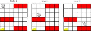
In egocentric learning, each situation is determined by what is near the mouse, and so new action values for each of the possible movements ({W,NW,N,NE,E,SE,S,SW}) have to be learned whenever the immediate environment is not something the agent has seen before. For example, the mouse keeps a different set of action values for each of the following environments:

On the other hand, in the case of allocentric learning, each situation is determined by the (x,y) coordinates of the mouse’s current position. That means that the mouse keeps a different set of action values for every possible (x,y) position:

so even if the environment in each position is the same:

with different (x,y) coordinates the mouse maintains different action value maps for all of them.

With egocentric learning, the agent tends to develop immediately beneficial behavior more quickly, to avoid running off cliffs and to move towards cheese when it’s in sight. The agent can even learn to move towards cheese that’s outside of the range of its sensors in simple maps, essentially by learning heuristics like ‘always moving right leads to reward.’ But this falls apart if there are several areas in the map where the immediate environment is the same, as in the case above with states 2 and 3.

With allocentric learning, the agent develops action value mappings that are much better suited to the overall environment and long-term goals (e.g. if the cheese is always in the center of the map, if you are in the bottom-right move up and left, and if you are in the top-left move down and right), but you can’t generalize across local situations (for example when there is a cliff one space to the right), the consequences of movement at each (x,y) position must be learned independently.

Clearly a combination of these two learning types is desirable, but that is for a future post! There is still a lot to examine in ego-centric learning, and so we’re going to dig deeper.

Thinking about the future

In allocentric learning, you don’t often perform an action, successfully move, and then still wind up in the same state. This makes transmitting information about rewards received in the future backwards to states that are still far away fairly stable, because a specific state is some constant distance away from getting reward. In egocentric learning, however, this isn’t the case. So when you start trying to propagate reward information backwards you can get some unstable behavior; let’s look at a very basic scenario:

There’s the mouse in blue, on the left, and the reward, in green, on the right, and red represents cliffs / certain death. So now, whenever the mouse isn’t beside one of the walls he will be in one of three states, cliffs above, nothing around him, or cliffs below:

OK. Now let’s look at the update formula for Q-learning again:

Q(s, a) += alpha * (reward(s') + gamma * max(Q(s')) - Q(s, a))

where s is the previous system state, a is the action just taken, s' is the current state, reward(s') is the reward for being in the current state, and max(Q(s')) is the maximum reward obtainable by performing an action in the current state.

Informally, it says that the change to make to the Q-value for the action just taken, Q(s, a), is equal to your learning rate, alpha, multiplied by the reward for the state that you moved into,reward(s'), plus the lookahead reward,max(Q(s')), which relays the expected reward now that you’re in state s', minus the previous Q-value,Q(s, a).

Let’s break this down a bit more, because this can be complicated to think about still. If we set gamma = 0, then our update is

Q(s, a) += alpha * (reward(s') - Q(s, a)).

Here it’s more apparent what the dynamics are doing, they’re driving the Q-value to the reward value of the state you end up in. So you take an action a in state s, you find the reward for where you ended up, and you learn the reward for performing action a in state s. Now if gamma is not equal to 0, then you can think of the Q-value dynamics as trying to drive the Q-values to

reward(s') + gamma * max(Q(s'))

The larger that gamma is, the farther into the future you look. This can lead to unstable / non-convergent systems when you repeatedly move into the same state again and again. For example, if you’re in State 2 from above, and you move right often enough you’ll end up in a state that leads to getting a reward. This boosts the state before the reward, and now the next time you happen to move to a state where the reward is next to you, the Q-values of State 2 are now updated. And so you get your reward and you reset. Now you move into State 2 again and hey! Moving right leads to a reward. So you move right, but now you’re back in State 2 again! And so the reward for moving right decreases a bit. But it’s still the best decision, so you move right. And you’re in State 2 again, and so the reward for moving right goes down again, etc etc. Eventually moving right brings you to the target though and the Q-value for moving right gets a boost. So it’s going to forever be fluctuating.

In this example, it doesn’t seem like a big deal, because the mouse still learns to move towards the cheese and the Q-values have entered a kind of rhythmic limit cycle. There are a few problems that arise, however, when counting the future to heavily in egocentric learning.

Problem: Death-wish

Basically, the mouse decides that certain death is a better option than wandering around in uncertainty forever and starts deciding to commit suicide. Let’s say that to encourage exploration, the reward for being in an unoccupied square is -1, and to encourage not dying the reward for jumping off a cliff is -10. The problem arises in that jumping off the cliff is a constant punishment, -10. It’s always -10 and it will never be any worse than -10. There is no further future past death to influence the reward. When the mouse is just exploring, however, it will explore, and get -1, and then explore more, and get -1, etc etc. This causes the expected reward of actions that lead you into the same state keep dropping. If the weight of gamma is too large, then without all that much exploring the reward for exploring has suddenly dropped to less than -10, and the mouse decides that continuing to explore is worse than death, and jumps.

By setting gamma = 5 (which is pretty high) we then get this behavior very quickly, here are some simulation results, where the first column is the timestep, the second column W denotes how many times the mouse found the cheese, the third column L denotes how many times the mouse chose to jump off a cliff (as dictated by its Q-values), and the last column A denotes how many times random exploration led the mouse to its accidental death:

10000, W: 0, L: 3138, A: 51
20000, W: 0, L: 3207, A: 40
30000, W: 0, L: 3204, A: 40
40000, W: 0, L: 3205, A: 45
50000, W: 0, L: 3208, A: 43
60000, W: 0, L: 3198, A: 49
70000, W: 0, L: 3200, A: 49
80000, W: 0, L: 3207, A: 46
90000, W: 0, L: 3204, A: 46
100000, W: 0, L: 3214, A: 38
110000, W: 0, L: 3211, A: 37
120000, W: 0, L: 3203, A: 44
130000, W: 0, L: 3199, A: 45
140000, W: 0, L: 3225, A: 28
150000, W: 0, L: 3211, A: 39
160000, W: 0, L: 3196, A: 45
170000, W: 0, L: 3208, A: 46
180000, W: 0, L: 3203, A: 47
190000, W: 0, L: 3209, A: 38
200000, W: 0, L: 3216, A: 38

So pretty immediately the mouse gets into a dark place, and starts choosing to jump, without ever having found the cheese even once.

Problem: Confusion

Another problem is that by heavily weighting the immediate future the mouse can get easily confused again about what was good or how it actually found the cheese and got the big reward in the first place. Once State 2 has rewarded moving right, and the mouse moves left, there is now a new max(Q(s')) value for State 2 (the reward for moving right), and so the reward for moving left is now brought up. At the same time, the reward for moving right is dropping every time it moves right and doesn’t get rewarded (as described above). Same with moving up and down, so very quickly the Q-values can be flooded with high values and the optimal direction of movement is lost.

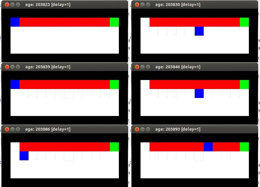
We can see this case by setting gamma = .8. Now, the mouse will find the cheese and learns to move right, but there are also these blips of confusion where it forgets how to find the cheese,

10000, W: 0, L: 4, A: 78
20000, W: 0, L: 0, A: 78
30000, W: 87, L: 0, A: 67
40000, W: 810, L: 0, A: 16
50000, W: 841, L: 0, A: 1
60000, W: 843, L: 0, A: 2
70000, W: 847, L: 0, A: 3
80000, W: 816, L: 0, A: 10
90000, W: 667, L: 0, A: 17
100000, W: 0, L: 0, A: 68
110000, W: 0, L: 0, A: 68
120000, W: 34, L: 0, A: 68
130000, W: 748, L: 0, A: 43
140000, W: 853, L: 0, A: 0
150000, W: 846, L: 0, A: 2
160000, W: 847, L: 0, A: 3
170000, W: 856, L: 0, A: 2
180000, W: 853, L: 0, A: 2
190000, W: 120, L: 0, A: 62
200000, W: 0, L: 0, A: 70

So it’s getting there, but then it gets confused and forgets how to find it, then it remembers, then it forgets…etc.

Solution: Have a healthy fear of death

If instead now we set gamma = .05, the mouse has a much stronger repulsion to imminent death than to ennui for a much longer time, and will go around exploring things (note that this is the same as changing the reward for dying to be a much higher penalty). As a result the mouse will find the cheese faster. As a bonus, we also don’t have the fits of forgetfulness seem in the previous example:

10000, W: 313, L: 4, A: 50
20000, W: 845, L: 0, A: 6
30000, W: 848, L: 0, A: 1
40000, W: 850, L: 0, A: 1
50000, W: 850, L: 0, A: 1
60000, W: 846, L: 0, A: 2
70000, W: 844, L: 0, A: 6
80000, W: 843, L: 0, A: 2
90000, W: 846, L: 0, A: 2
100000, W: 847, L: 0, A: 5
110000, W: 844, L: 0, A: 4
120000, W: 849, L: 0, A: 3
130000, W: 846, L: 0, A: 5
140000, W: 842, L: 0, A: 4
150000, W: 845, L: 0, A: 4
160000, W: 847, L: 0, A: 5
170000, W: 848, L: 0, A: 10
180000, W: 844, L: 0, A: 7
190000, W: 840, L: 0, A: 8
200000, W: 848, L: 0, A: 1

And so in this case now we’ve developed a pretty good, stable, egocentric RL mouse, that can learn to avoid jumping off cliffs and find the cheese in this very simple map.

We can still, of course, drop the gamma value down to the extreme, 0, such that our egocentric learner would have no knowledge of any future further than the reward it gets for taking the next step. In this case it would know that going off a cliff is bad, but it won’t know that moving to the right will eventually lead to cheese / a reward.

However, that can be OK! Warding off any immediate danger is and capitalizing on any immediate reward is the perfect role for this kind of short-sighted system. Trying to make it learn how to run through a complicated maze without a lot of very specific landmarks is just not something that’s going to happen.

Conclusions

So, recapping, the egocentric system learns Q-values for states that are based on the environment relative to the agent. This has some important consequences, in that it allows it to learn very quickly not to move forward if there’s a cliff in front of you, and that if there’s a reward in the immediate vicinity to go get it. Setting the weight on the expected reward in the Q-values update can lead to some unstable behavior, and it’s important to have a good concept of how the behavior of the agent changes with different gamma values. These undesirable behaviors can be avoided by setting gamma = 0, but the agent will then only learn the consequences of its immediate action, and be unable to look into the future at all to see how to bring about a reward or avoid getting trapped.

The egocentric learner has strengths where the allocentric learner fails, and the allocentric learner has strengths where the egocentric learner fails. The natural thought is to combine these two learners, and that will be the subject of the next RL post!

Reinforcement Learning part 2: SARSA vs Q-learning

In my previous post about reinforcement learning I talked about Q-learning, and how that works in the context of a cat vs mouse game. I mentioned in this post that there are a number of other methods of reinforcement learning aside from Q-learning, and today I’ll talk about another one of them: SARSA. All the code used is from Terry Stewart’s RL code repository, and can be found both there and in a minimalist version on my own github: SARSA vs Qlearn cliff. To run the code, simply execute the cliff_Q or the cliff_S files.

SARSA stands for State-Action-Reward-State-Action. In SARSA, the agent starts in state 1, performs action 1, and gets a reward (reward 1). Now, it’s in state 2 and performs another action (action 2) and gets the reward from this state (reward 2) before it goes back and updates the value of action 1 performed in state 1. In contrast, in Q-learning the agent starts in state 1, performs action 1 and gets a reward (reward 1), and then looks and sees what the maximum possible reward for an action is in state 2, and uses that to update the action value of performing action 1 in state 1. So the difference is in the way the future reward is found. In Q-learning it’s simply the highest possible action that can be taken from state 2, and in SARSA it’s the value of the actual action that was taken.

This means that SARSA takes into account the control policy by which the agent is moving, and incorporates that into its update of action values, where Q-learning simply assumes that an optimal policy is being followed. This difference can be a little difficult conceptually to tease out at first but with an example will hopefully become clear.

Mouse vs cliff

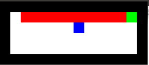
Let’s look at a simple scenario, a mouse is trying to get to a piece of cheese. Additionally, there is a cliff in the map that must be avoided, or the mouse falls, gets a negative reward, and has to start back at the beginning. The simulation looks something like exactly like this:

where the black is the edge of the map (walls), the red is the cliff area, the blue is the mouse and the green is the cheese. As mentioned and linked to above, the code for all of these examples can be found on my github (as a side note: when using the github code remember that you can press the page-up and page-down buttons to speed up and slow down the rate of simulation!)

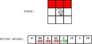
Now, as we all remember, in the basic Q-learning control policy the action to take is chosen by having the highest action value. However, there is also a chance that some random action will be chosen; this is the built-in exploration mechanism of the agent. This means that even if we see this scenario:

There is a chance that that mouse is going to say ‘yes I see the best move, but…the hell with it’ and jump over the edge! All in the name of exploration. This becomes a problem, because if the mouse was following an optimal control strategy, it would simply run right along the edge of the cliff all the way over to the cheese and grab it. Q-learning assumes that the mouse is following the optimal control strategy, so the action values will converge such that the best path is along the cliff. Here’s an animation of the result of running the Q-learning code for a long time:

The solution that the mouse ends up with is running along the edge of the cliff and occasionally jumping off and plummeting to its death.

However, if the agent’s actual control strategy is taken into account when learning, something very different happens. Here is the result of the mouse learning to find its way to the cheese using SARSA:

Why, that’s much better! The mouse has learned that from time to time it does really foolish things, so the best path is not to run along the edge of the cliff straight to the cheese but to get far away from the cliff and then work its way over safely. As you can see, even if a random action is chosen there is little chance of it resulting in death.

Learning action values with SARSA

So now we know how SARSA determines it’s updates to the action values. It’s a very minor difference between the SARSA and Q-learning implementations, but it causes a profound effect.

Here is the Q-learning learn method:

def learn(self, state1, action1, reward, state2):
    maxqnew = max([self.getQ(state2, a) for a in self.actions])
    self.learnQ(state1, action1,
                reward, reward + self.gamma*maxqnew)

And here is the SARSA learn method

def learn(self, state1, action1, reward, state2, action2):
    qnext = self.getQ(state2, action2)
    self.learnQ(state1, action1,
                reward, reward + self.gamma * qnext)

As we can see, the SARSA method takes another parameter, action2, which is the action that was taken by the agent from the second state. This allows the agent to explicitly find the future reward value, qnext, that followed, rather than assuming that the optimal action will be taken and that the largest reward, maxqnew, resulted.

Written out, the Q-learning update policy is Q(s, a) = reward(s) + alpha * max(Q(s')), and the SARSA update policy is Q(s, a) = reward(s) + alpha * Q(s', a'). This is how SARSA is able to take into account the control policy of the agent during learning. It means that information needs to be stored longer before the action values can be updated, but also means that our mouse is going to jump off a cliff much less frequently, which we can probably all agree is a good thing.

Online Goal Babbling – motor learning paper review

Recently I was linked to an article about learning how to control a highly complex arm from scratch: How infants tell us how to control the Bionic Handling Assistant. The work seemed very interesting so I went and pulled one of the papers linked in the article, Online Goal Babbling for rapid bootstrapping of inverse models in high dimensions.

Diving into that title, online means that we’re using information from every movement as it’s gathered to improve our control, as opposed to ‘batch’ where learning only occurs every so-many trials. Bootstrapping is the process of bringing a system up to a functionally useful level. High dimensions then refers to the complexity of the system being controlled, where every component that requires a control signal is another dimension. Humans, for example, require extremely high dimensional control signals. Inverse models refer to a type of internal model, which ‘describe relations between motor commands and their consequences’. Forward models predict the results of a movement, and inverse models allow suggest a motor command that can be used to achieve a desired consequence, such as ‘the ball falls on the floor’ or ‘my hand touches the red balloon’.

Alright, so that’s the title, let’s dive into the paper proper.

Online goal babbling

The idea behind this research is to let the system learn how to control itself by exploring the environment. The reason why you would want to do this is so that you don’t have to analytically specify how the system should move. Analytic solutions require accurate models of the system dynamics, and calculating these quickly become horrendously complex. To the point that the equations of motion for a relatively simple 3-link arm moving are pages upon pages upon pages. On top of this, because your solution is only is as good as your model and the model you just took all that time to calculate isn’t adaptive, if your system dynamics change at all through wear and tear or an environment change, you’re in big trouble. You can use feedback control to help compensate for the errors introduced, but you can only respond as fast as you can receive and process sensory signals, which is often too long in practical applications.

So this moves us to adaptive feedforward control, based on learning an inverse model of the system dynamics. Importantly, what this paper describes is a kinematic inverse controller, not a kinetic inverse controller; meaning that given a desired target position for the end effector (hand) of an arm it provides a sequence of joint angle sets that will lead to the end effector reaching the target, as opposed to providing a sequence of joint angle torques to drive the system to the target. At some point, a control system will have to generate force commands, rather than just specify what position it wants the system to be in. But, knowing what joint angles and trajectory the joint angles should follow is an important problem, because systems that are of interest to control tend to exhibit a fair amount of configuration redundancy between ‘task-space’ and the actual system state-space. Task-space being something like the 3-dimensional position of the end-effector, which we are interested in controlling, and the actual system state-space being something like the joint-angles or muscle-lengths. Configuration redundancy is the problem of more than one possible set of joint-angles putting the end-effector in the desired location. Often the number of potential solutions is incredibly large, think about the number of possible ways you can reach to an object. So how do you learn an appropriate trajectory for your joint angles during a reaching movement? That is the problem being addressed here.

To learn an inverse model from scratch, the system needs to explore. How should it explore? Moving randomly eventually leads to an exhaustive search, but this is a poor choice in complex systems because it takes a large amount of time, increasing exponentially with the degrees of freedom (i.e. number of joint angles) of the system. So let’s look to babies, they’re responsible for learning how to control a very complex system, how the heck do they learn to move?

‘Motor babbling’ is a term that was coined to describe the seemingly random way babies moved about. It was suggested that they just flail about without purpose until they gain some understanding of how their bodies work, at which point they can start moving with purpose. But! Baby movement was shown way back in the 80’s to in fact not be just random, but instead to be highly goal directed. And when they find a solution, they stick with it, they don’t worry about it being the best one as long as it gets the job done. Only later are movements tweaked to be more efficient. As mentioned above, in systems as complicated as the human body the task-space (i.e. position of the hand) is much smaller than the motor space (i.e. length of all muscles), and there are a bunch of different solutions to a given task. With all these different potential solutions to a given problem, an exhaustive search isn’t even close to being necessary. Also, if babies aren’t just randomly exploring space to figure things out, they don’t have to flip a switch somewhere in their brain that says “ok stop messing around and let’s move with purpose”.

This paper provides a technique for stable online inverse model learning that can be used from initial bootstrapping, and shows how online learning can even be highly beneficial for bootstrapping. So let’s dive into the Online Goal Babbling learning method.

The inverse model function

Let’s denote the inverse model function we’re learning as , joint angles as , and end effector positions as . Then to denote giving a desired end effector position and getting out a set of joint angles we write , where represents a target in end effector space.

We’re going to initialize the inverse model function by having every end effector position return some default resting state of the arm, or home position, that we’ve defined, . Additionally, we’re going to throw on some exploratory noise to the answer provided by the inverse model, so that the joint angles to move to at time are defined as , where is the exploratory noise. When the system then moves to the end effector position, , is observed and the parameters of the inverse model, , are updated immediately.

To generate a smooth path from the starting position to the target, the system divides the distance up into a number of sub-targets (25 in the paper) for the system to hit along the way. This is an important point, as it’s how the inverse model function is used to create a path that represents the system moving; a series of targets are provided and the inverse model is queried “what should the joint configuration be for this position?”

As mentioned before, it is possible to have he end effector in the same position, but the joints in a different configuration. Learning across these examples is dangerous and can lead to instability in the system as neighbouring targets could be learned with very dissimilar joint configurations, preventing smooth movement through joint-space. To prevent this, observed information is weighted by a term as it is taken in, based on deviation from the resting position of the arm () and efficiency of end effector movement. What this leads to is a consistent solution to be converged upon throughout movement space, causing the inverse model to generate smooth, comfortable (i.e. not near joint limits, but near the resting state of the arm) movements.

Additions to movement commands

To recenter movement exploration every so often, and prevent the system from exploring heavily in some obscure joint-space, every time a new target to move to is selected there is some probability (.1 in the paper) that the system will return to . To return home the system traces out a straight trajectory in joint-space, not worrying about how it is moving through end effector space. This return probability reinforces learning how to move well near , and acts as a ‘developmentally plausible stabilizer that helps to stay on known areas of the sensorimotor space.’

Also, we mentioned adding exploratory noise. How is that noise generated? The noise is calculated through a small, randomly chosen linear function that varies slowly over time: , where the entries to the matrix and vector are chosen independently from a normal distribution with zero mean and variance . To move, a set of small values is chosen from a normal distribution with variance significantly smaller than , and added to elements of and . A normalization term is also used to keep the overall deviation stable around the standard deviation . And that’s how we get our slowly changing linear random noise function.

Online learning

To learn the inverse model function, we’re going to use the technique of creating a bunch of linear models that are accurate in a small area of state space, and weighting their contribution to the output based on how close we are to their ‘region of validity’. The specific method used in the paper is a local-linear map, from (H.Ritter, Learning with the self-organizing map 1991). We define our linear models as , intuited as following the standard definition of a line, but moving into multiple dimensions. is our linear transformation of the input for model , and is the offset.

If an input is received that is outside of the region of validity for all of the local linear models, then another one is added to improve the approximation of the function at that point. New local models are initiated with the Jacobian matrix of the inverse estimate. In other words, we look at how the approximation of the function is changing as we move in this direction in state space, or estimate the derivative of the function, and use that to set the initial value of our new linear model.

To update our inverse model function, we fit it to the current example by reducing the weighted square error: . With this error, a standard gradient descent method is used to update the slopes and offsets of the dimensions of the linear models:

,

where is the learning rate.

Results

So here are some figures of the results of applying the algorithm, and they’re pretty impressive. First we see learning the inverse model for a 5-link arm:

And one of the really neat things about this is the scalability of this algorithm. Here’s applying OGB to a 50-link arm:

And here are some results looking at varying the learning rate (x-axis) and the effects on (a) time until 10% error reached, (b) final performance error, and (c) final average distance from , the resting state configuration.

Comments and thoughts

I enjoyed reading this paper, although I thought the ‘Learning operational space control’ papers from Jan Peters and Stephen Schaal deserved a bit more of a shout-out, as they’ve been around since 2006/8 and it’s a very similar method. Also I pulled one of the older papers from the article, so I’ll need to review the other ones too soon, as there is clearly more going on for the successful control of the elephant trunk arm shown in the article.

Other than that, I’m a big fan of breaking up complicated, non-linear functions into a bunch of small linear models, and stitching them all back together to learn an accurate approximation. I think it’s a very likely candidate for the kind of way that the brain goes about learning these incredibly complicated models, especially in the cerebellum I hold these types of methods as a favorite for how biological systems accomplish this. Another important note is that the learning never ‘turns off’ here, which is another big plus to this method. It allows the system to converge upon a solution, but to keep exploring the space as it uses this solution, so more efficient solutions can be found. Additionally, this makes this system much more robust to changing dynamics, resultant of wear and tear or, as in the case of infants, growing.

Again, the model here is learning an kinematic control of the system, specifying what joint angles the system should move to, and not the joint torques that will be required to actually move the system there. But, I am partial to the idea that this kinematic inverse model does then make it a much more smooth function for the kinetic controller to learn from this point.

The way I picture it is specifying a target in end-effector space, learning an kinematic inverse model controller that can specify the appropriate joint trajectory to follow to reach this target. Then an kinetic inverse model controller that takes in the joint space path, looks at the current joint angles / velocities / and accelerations, and learns the appropriate torques or muscle activation commands to move the arm as desired. This is a much, much smoother function to learn than directly learning the appropriate joint torques for a desired target in end effector space, because there are no hidden configuration redundancies. It’s still complex, because it still has to compensate for the inertia and multi-link interaction dynamics, but should still hopefully be much more straight-forward to learn.

Rolf, Matthias. (2011). Online Goal Babbling for rapid bootstrapping of inverse models in high dimensions. Development and Learning (ICDL), 2011 IEEE DOI: 10.1109/DEVLRN.2011.6037368

claimtoken-511bf485684de

Reinforcement learning part 1: Q-learning and exploration

We’ve been running a reading group on Reinforcement Learning (RL) in my lab the last couple of months, and recently we’ve been looking at a very entertaining simulation for testing RL strategies, ye’ old cat vs mouse paradigm. There are a number of different RL methods you can use / play with in that tutorial, but for this I’m only going to talk about Q-learning. The code implementation I’ll be using is all in Python, and the original code comes from one of our resident post-docs, Terry Stewart, and can be garnered from his online RL tutorial. The code I modify here is based off of Terry’s code and modified by Eric Hunsberger, another PhD student in my lab. I’ll talk more about how it’s been modified in another post.

Q-learning review
For those unfamiliar, the basic gist of Q-learning is that you have a representation of the environmental states s, and possible actions in those states a, and you learn the value of each of those actions in each of those states. Intuitively, this value, Q, is referred to as the state-action value. So in Q-learning you start by setting all your state-action values to 0 (this isn’t always the case, but in this simple implementation it will be), and you go around and explore the state-action space. After you try an action in a state, you evaluate the state that it has lead to. If it has lead to an undesirable outcome you reduce the Q value (or weight) of that action from that state so that other actions will have a greater value and be chosen instead the next time you’re in that state. Similarly, if you’re rewarded for taking a particular action, the weight of that action for that state is increased, so you’re more likely to choose it again the next time you’re in that state. Importantly, when you update Q, you’re updating it for the previous state-action combination. You can only update Q after you’ve seen what results.

Let’s look at an example in the cat vs mouse case, where you are the mouse. You were in the state where the cat was in front of you, and you chose to go forward into the cat. This caused you to get eaten, so now reduce the weight of that action for that state, so that the next time the cat is in front of you you won’t choose to go forward you might choose to go to the side or away from the cat instead (you are a mouse with respawning powers). Note that this doesn’t reduce the value of moving forward when there is no cat in front of you, the value for ‘move forward’ is only reduced in the situation that there’s a cat in front of you. In the opposite case, if there’s cheese in front of you and you choose ‘move forward’ you get rewarded. So now the next time you’re in the situation (state) that there’s cheese in front of you, the action ‘move forward’ is more likely to be chosen, because last time you chose it you were rewarded.

Now this system, as is, gives you no foresight further than one time step. Not incredibly useful and clearly too limited to be a real strategy employed in biological systems. Something that we can do to make this more useful is include a look-ahead value. The look-ahead works as follows. When we’re updating a given Q value for the state-action combination we just experienced, we do a search over all the Q values for the state the we ended up in. We find the maximum state-action value in this state, and incorporate that into our update of the Q value representing the state-action combination we just experienced.

For example, we’re a mouse again. Our state is that cheese is one step ahead, and we haven’t learned anything yet (blank value in the action box represents 0). So we randomly choose an action and we happen to choose ‘move forward’.
Now, in this state (we are on top of cheese) we are rewarded, and so we go back and update the Q value for the state ‘cheese is one step ahead’ and the action ‘move forward’ and increase the value of ‘move forward’ for that state.
Now let’s say the cheese is moved and we’re moving around again, now we’re in the state ‘cheese is two steps ahead’, and we make a move and end up in the state ‘cheese is one step ahead’.
Now when we are updating the Q value for the previous state-action combination we look at all the Q values for the state ‘cheese is one step ahead’. We see that one of these values is high (this being for the action ‘move forward’) and this value is incorporated in the update of the previous state-action combination.
Specifically we’re updating the previous state-action value using the equation: Q(s, a) += alpha * (reward(s,a) + max(Q(s') - Q(s,a)) where s is the previous state, a is the previous action, s' is the current state, and alpha is the discount factor (set to .5 here).

Intuitively, the change in the Q-value for performing action a in state s is the difference between the actual reward (reward(s,a) + max(Q(s'))) and the expected reward (Q(s,a)) multiplied by a learning rate, alpha. You can think of this as a kind of PD control, driving your system to the target, which is in this case the correct Q-value.

Here, we evaluate the reward of moving ahead when the cheese is two steps ahead as the reward for moving into that state (0), plus the reward of the best action from that state (moving into the cheese +50), minus the expected value of that state (0), multiplied by our learning rate (.5) = +25.

Exploration
In the most straightforward implementation of Q-learning, state-action values are stored in a look-up table. So we have a giant table, which is size N x M, where N is the number of different possible states, and M is the number of different possible actions. So then at decision time we simply go to that table, look up the corresponding action values for that state, and choose the maximum, in equation form:

def choose_action(self, state):
    q = [self.getQ(state, a) for a in self.actions]
    maxQ = max(q)
    action = self.actions[maxQ]
    return action

Almost. There are a couple of additional things we need to add. First, we need to cover the case where there are several actions that all have the same value. So to do that, if there are several with the same value, randomly choose one of them.

def choose_action(self, state):
    q = [self.getQ(state, a) for a in self.actions]
    maxQ = max(q)
    count = q.count(maxQ)
    if count > 1:
        best = [i for i in range(len(self.actions)) if q[i] == maxQ]
        i = random.choice(best)
    else:
        i = q.index(maxQ)

    action = self.actions[i]
    return action

This helps us out of that situation, but now if we ever happen upon a decent option, we’ll always choose that one in the future, even if there is a way better option available. To overcome this, we’re going to need to introduce exploration. The standard way to get exploration is to introduce an additional term, epsilon. We then randomly generate a value, and if that value is less than epsilon, a random action is chosen, instead of following our normal tactic of choosing the max Q value.

def choose_action(self, state):
    if random.random() < self.epsilon: # exploration action = random.choice(self.actions) else: q = [self.getQ(state, a) for a in self.actions] maxQ = max(q) count = q.count(maxQ) if count > 1:
            best = [i for i in range(len(self.actions)) if q[i] == maxQ]
            i = random.choice(best)
        else:
            i = q.index(maxQ)

       action = self.actions[i]
    return action

The problem now is that we even after we’ve explored all the options and we know for sure the best option, we still sometimes choose a random action; the exploration doesn’t turn off. There are a number of ways to overcome this, most involving manually adjusting epsilon as the mouse learns, so that it explores less and less as time passes and it has presumably learned the best actions for the majority of situations. I’m not a big fan of this, so instead I’ve implemented exploration the following way: If the randomly generated value is less than epsilon, then randomly add values to the Q values for this state, scaled by the maximum Q value of this state. In this way, exploration is added, but you’re still using your learned Q values as a basis for choosing your action, rather than just randomly choosing an action completely at random.

    def choose_action(self, state):
        q = [self.getQ(state, a) for a in self.actions]
        maxQ = max(q)

        if random.random()  1:
            best = [i for i in range(len(self.actions)) if q[i] == maxQ]
            i = random.choice(best)
        else:
            i = q.index(maxQ)

        action = self.actions[i]

        return action

Very pleasingly, you get results comparable to the case where you perform lots of learning and then set epsilon = 0 to turn off random movements. Let’s look at them!

Simulation results
So here, the simulation is set up such that there is a mouse, cheese, and a cat all inside a room. The mouse then learns over a number of trials to avoid the cat and get the cheese. Printing out the results after every 1,000 time steps, for the standard learning case where you reduce epsilon as you learn the results are:

10000, e: 0.09, W: 44, L: 778
20000, e: 0.08, W: 39, L: 617
30000, e: 0.07, W: 47, L: 437
40000, e: 0.06, W: 33, L: 376
50000, e: 0.05, W: 35, L: 316
60000, e: 0.04, W: 36, L: 285
70000, e: 0.03, W: 33, L: 255
80000, e: 0.02, W: 31, L: 179
90000, e: 0.01, W: 35, L: 152
100000, e: 0.00, W: 44, L: 130
110000, e: 0.00, W: 28, L: 90
120000, e: 0.00, W: 17, L: 65
130000, e: 0.00, W: 40, L: 117
140000, e: 0.00, W: 56, L: 86
150000, e: 0.00, W: 37, L: 77

For comparison now, here are the results when epsilon is not reduced in the standard exploration case:

10000, e: 0.10, W: 53, L: 836
20000, e: 0.10, W: 69, L: 623
30000, e: 0.10, W: 33, L: 452
40000, e: 0.10, W: 32, L: 408
50000, e: 0.10, W: 57, L: 397
60000, e: 0.10, W: 41, L: 326
70000, e: 0.10, W: 40, L: 317
80000, e: 0.10, W: 47, L: 341
90000, e: 0.10, W: 47, L: 309
100000, e: 0.10, W: 54, L: 251
110000, e: 0.10, W: 35, L: 278
120000, e: 0.10, W: 61, L: 278
130000, e: 0.10, W: 45, L: 295
140000, e: 0.10, W: 67, L: 283
150000, e: 0.10, W: 50, L: 304

As you can see, the performance now converges around 300, instead of 100. Not great.
Now here are the results from the alternative implementation of exploration, where epsilon is held constant:

10000, e: 0.10, W: 65, L: 805
20000, e: 0.10, W: 36, L: 516
30000, e: 0.10, W: 50, L: 417
40000, e: 0.10, W: 38, L: 310
50000, e: 0.10, W: 39, L: 247
60000, e: 0.10, W: 31, L: 225
70000, e: 0.10, W: 23, L: 181
80000, e: 0.10, W: 34, L: 159
90000, e: 0.10, W: 36, L: 137
100000, e: 0.10, W: 35, L: 138
110000, e: 0.10, W: 42, L: 136
120000, e: 0.10, W: 24, L: 99
130000, e: 0.10, W: 52, L: 106
140000, e: 0.10, W: 22, L: 88
150000, e: 0.10, W: 29, L: 101

And again we get that nice convergence to 100, but this time without having to manually modify epsilon. Which is pretty baller.

Code
And that’s it! There is of course lots and lots of other facets of exploration to discuss, but this is just a brief discussion. If you’d like the code for the cat vs mouse and the alternative exploration you can access them at my github: Cat vs mouse – exploration.
To alternate between the different types of exploration, change the import statement at the top of the egoMouseLook.py to be either import qlearn for the standard exploration method, or import qlearn_mod_random as qlearn to test the alternative method. To have epsilon reduce in value as time goes, you can uncomment the lines 142-145.