About a year ago I published the work from my thesis in a paper called ‘A spiking neural model of adaptive arm control’. In this paper I presented the Recurrent Error-driven Adaptive Control Hierarchy (REACH) model. The goal of the model is to begin working towards reproducing behavioural level phenomena of human movement with biologically plausible spiking neural networks.
To do this, I start by using three methods from control literature (operational space control, dynamic movement primitives, and non-linear adaptive control) to create an algorithms level model of the motor control system that captures behavioural level phenomena of human movement. Then I explore how this functionality could be mapped to the primate brain and implemented in spiking neurons. Finally, I look at the data generated by this model on the behavioural level (e.g. kinematics of movement), the systems level (i.e. analysis of populations of neurons), and the single-cell level (e.g. correlating neural activity with movement parameters) and compare/contrast with experimental data.
By having a full model framework (from observable behaviour to neural spikes) is to have a more constrained computational model of the motor control system; adding lower-level biological constraints to behavioural models and higher-level behavioural constraints to neural models.
In general, once you have a model, the critical next step is to generating testable predictions that can be used to discriminate between other models with different implementations or underlying algorithms. Discriminative predictions allow us to design experiments that can gather evidence in favour or against different hypotheses of brain function, and provide clues to useful directions for further research. Which is the real contribution of computational modeling.
So that’s a quick overview of the paper; there are quite a few pages of supplementary information that describe the details of the model implementation, and I provided the code and data used to generate the data analysis figures. However, code to explicitly run the model on your own has been missing. As one of the major points of this blog is to provide code for furthering research, this is pretty embarrassing. So, to begin to remedy this, in this post I’m going to work through a REACH framework for building models to control a two-link arm through reaching in a line, tracing a circle, performing the centre-out reaching task, and adapting online to unexpected perturbations during reaching imposed by a joint-velocity based forcefield.
This post is directed towards those who have already read the paper (although not necessarily the supplementary material). To run the scripts you’ll need Nengo, Nengo GUI, and NengoLib all installed. There’s a description of the theory behind the Neural Engineering Framework, which I use extensively in my Nengo modeling, in the paper. I’m hoping that between that and code readability / my explanations below that most will be comfortable starting to play around with the code. But if you’re not, and would like more resources, you can check out the Getting Started page on the Nengo website, the tutorials from How To Build a Brain, and the examples in the Nengo GUI.
You can find all of the code up on my GitHub.
NOTE: I’m using the two-link arm (which is fully implemented in Python) instead of the three-link arm (which has compile issues for Macs) both so that everyone should be able to run the model arm code and to reduce the number of neurons that are required for control, so that hopefully you can run this on you laptop in the event that you don’t have a super power Ubuntu work station. Scaling this model up to the three-link arm is straight-forward though, and I will work on getting code up (for the three-link arm for non-Mac users) as a next project.
Implementing PMC – the trajectory generation system
I’ve talked at length about dynamic movement primitives (DMPs) in previous posts, so I won’t describe those again here. Instead I will focus on their implementation in neurons.
def generate(y_des, speed=1, alpha=1000.0):
    beta = alpha / 4.0

    # generate the forcing function
    forces, _, goals = forcing_functions.generate(
        y_des=y_des, rhythmic=False, alpha=alpha, beta=beta)

    # create alpha synapse, which has point attractor dynamics
    tau = np.sqrt(1.0 / (alpha*beta))
    alpha_synapse = nengolib.Alpha(tau)

    net = nengo.Network('PMC')
    with net:
        net.output = nengo.Node(size_in=2)

        # create a start / stop movement signal
        time_func = lambda t: min(max(
            (t * speed) % 4.5 - 2.5, -1), 1)

        def goal_func(t):
            t = time_func(t)
            if t <= -1:
                return goals[0]
            return goals[1]
        net.goal = nengo.Node(output=goal_func, label='goal')

        # -------------------- Ramp ---------------------------
        ramp_node = nengo.Node(output=time_func, label='ramp')
        net.ramp = nengo.Ensemble(
            n_neurons=500, dimensions=1, label='ramp ens')
        nengo.Connection(ramp_node, net.ramp)

        # ------------------- Forcing Functions ---------------
        def relay_func(t, x):
            t = time_func(t)
            if t <= -1:
                return [0, 0]
            return x
        # the relay prevents forces from being sent on reset
        relay = nengo.Node(output=relay_func, size_in=2)

        domain = np.linspace(-1, 1, len(forces[0]))
        x_func = interpolate.interp1d(domain, forces[0])
        y_func = interpolate.interp1d(domain, forces[1])
        transform=1.0/alpha/beta
        nengo.Connection(net.ramp, relay[0], transform=transform,
                         function=x_func, synapse=alpha_synapse)
        nengo.Connection(net.ramp, relay[1], transform=transform,
                         function=y_func, synapse=alpha_synapse)
        nengo.Connection(relay, net.output)

        nengo.Connection(net.goal[0], net.output[0],
                         synapse=alpha_synapse)
        nengo.Connection(net.goal[1], net.output[1],
                         synapse=alpha_synapse)
    return net
The generate method for the PMC takes in a desired trajectory, y_des, as a parameter. The first thing we do (on lines 5-6) is calculate the forcing function that will push the DMP point attractor along the desired trajectory.
The next thing (on lines 9-10) is creating an Alpha (second-order low-pass filter) synapse. By writing out the dynamics of a point attractor in Laplace space, one of the lab members, Aaron Voelker, noticed that the dynamics could be fully implemented by creating an Alpha synapse with an appropriate choice of tau. I walk through all of the math behind this in this post. Here we’ll use that more compact method and project directly to the output node, which improves performance and reduces the number of neurons.
Inside the PMC network we create a time_func node, which is the pace-setter during simulation. It will output a linear ramp from -1 to 1 every few seconds, with the pace set by the speed parameter, and then pause before restarting.
We also have a goal node, which will provide a target starting and ending point for the trajectory. Both the time_func and goal nodes are created and used as a model simulation convenience, and proposed to be generated elsewhere in the brain (the basal ganglia, why not? #igotreasons #provemewrong).
The ramp ensemble is the most important component of the trajectory generation system. It takes the output from the time_func node as input, and generates the forcing function which will guide our little system through the trajectory that was passed in. The ensemble itself is nothing special, but rather the function that it approximates on its outgoing connection. We set up this function approximation with the following code:
        domain = np.linspace(-1, 1, len(forces[0]))
        x_func = interpolate.interp1d(domain, forces[0])
        y_func = interpolate.interp1d(domain, forces[1])
        transform=1.0/alpha/beta
        nengo.Connection(net.ramp, relay[0], transform=transform,
                         function=x_func, synapse=alpha_synapse)
        nengo.Connection(net.ramp, relay[1], transform=transform,
                         function=y_func, synapse=alpha_synapse)
        nengo.Connection(relay, net.output)
We want the forcing function be generated as the signals represented in the ramp ensemble moves from -1 to 1. To achieve this, we create interpolation functions, x_func and y_func, which are set up to generate the forcing function values mapped to input values between -1 and 1. We pass these functions into the outgoing connections from the ramp population (one for x and one for y). So now when the ramp ensemble is representing -1, 0, and 1 the output along the two connections will be the starting, middle, and ending x and y points of the forcing function trajectory. The transform and synapse are set on each connection with the appropriate gain values and Alpha synapse, respectively, to implement point attractor dynamics.
NOTE: The above DMP implementation can generate a trajectory signal with as many dimensions as you would like, and all that’s required is adding another outgoing Connection projecting from the ramp ensemble.
The last thing in the code is hooking up the goal node to the output, which completes the point attractor implementation.
Implementing M1 – the kinematics of operational space control
In REACH, we’ve modelled the primary motor cortex (M1) as responsible for taking in a desired hand movement (i.e. target_position - current_hand_position) and calculating a set of joint torques to carry that out. Explicitly, M1 generates the kinematics component of an OSC signal:

In the paper I did this using several populations of neurons, one to calculate the Jacobian, and then an EnsembleArray to perform the multiplication for the dot product of each dimension separately. Since then I’ve had the chance to rework things and it’s now done entirely in one ensemble.
Now, the set up for the M1 model that computes the above function is to have a single ensemble of neurons that takes in the joint angles,  , and control signal
  , and outputs the function above. Sounds pretty simple, right? Simple is good.
Let’s look at the code (where I’ve stripped out the comments and some debugging code):
def generate(arm, kp=1, operational_space=True,
             inertia_compensation=True, means=None, scales=None):

    dim = arm.DOF + 2

    means = np.zeros(dim) if means is None else means
    scales = np.ones(dim) if scales is None else scales
    scale_down, scale_up = generate_scaling_functions(
        np.asarray(means), np.asarray(scales))

    net = nengo.Network('M1')
    with net:
        # create / connect up M1 ------------------------------
        net.M1 = nengo.Ensemble(
            n_neurons=1000, dimensions=dim,
            radius=np.sqrt(dim),
            intercepts=AreaIntercepts(
                dimensions=dim,
                base=nengo.dists.Uniform(-1, .1)))

        # expecting input in form [q, x_des]
        net.input = nengo.Node(output=scale_down, size_in=dim)
        net.output = nengo.Node(size_in=arm.DOF)

        def M1_func(x, operational_space, inertia_compensation):
            """ calculate the kinematics of the OSC signal """
            x = scale_up(x)
            q = x[:arm.DOF]
            x_des = kp * x[arm.DOF:]

            # calculate hand (dx, dy)
            if operational_space:
                J = arm.J(q=q)

                if inertia_compensation:
                    # account for inertia
                    Mx = arm.Mx(q=q)
                    x_des = np.dot(Mx, x_des)
                # transform to joint torques
                u = np.dot(J.T, x_des)
            else:
                u = x_des

                if inertia_compensation:
                    # account for mass
                    M = arm.M(q=q)
                    u = np.dot(M, x_des)

            return u

        # send in system feedback and target information
        # don't account for synapses twice
        nengo.Connection(net.input, net.M1, synapse=None)
        nengo.Connection(
            net.M1, net.output,
            function=lambda x: M1_func(
                x, operational_space, inertia_compensation),
            synapse=None)

    return net
The ensemble of neurons itself is created with a few interesting parameters:
        net.M1 = nengo.Ensemble(
            n_neurons=1000, dimensions=dim,
            radius=np.sqrt(dim),
            intercepts=AreaIntercepts(
                dimensions=dim, base=nengo.dists.Uniform(-1, .1)))
Specifically, the radius and intercepts parameters.
Setting the intercepts
First we’ll discuss setting the intercepts using the AreaIntercepts distribution. The intercepts of a neuron determine how much of state space a neuron is active in, which we’ll refer to as the ‘active proportion’. If you don’t know what kind of functions you want to approximate with your neurons, then you having the active proportions for your ensemble chosen from a uniform distribution is a good starting point. This means that you’ll have roughly the same number of neurons active across all of state space as you do neurons that are active over half of state space as you do neurons that are active over very small portions of state space.
By default, Nengo sets the intercepts such that the distribution of active proportions is uniform for lower dimensional spaces. But when you start moving into higher dimensional spaces (into a hypersphere) the default method breaks down and you get mostly neurons that are either active for all of state space or almost none of state space. The AreaIntercepts class calculates how the intercepts should be set to achieve the desire active proportion inside a hypersphere. There are a lot more details here that you can read up on in this IPython notebook by Dr. Terrence C. Stewart.
What you need to know right now is that we’re setting the intercepts of the neurons such that the percentage of state space for which any given neuron is active is chosen from a uniform distribution between 0% and 55%. In other words, a neuron will maximally be active in 55% of state space, no more. This will let us model more nonlinear functions (such as the kinematics of the OSC signal) with fewer neurons. If this description is clear as mud, I really recommend checking out the IPython notebook linked above to get an intuition for what I’m talking about.
Scaling the input signal
The other parameter we set on the M1 ensemble is the radius. The radius scales the range of input values that the ensemble can represent, which is by default anything inside the unit hypersphere (i.e. hypersphere with radius=1). If the radius is left at this default value, the neural activity will saturate for vectors with magnitude greater than 1, leading to inaccurate vector representation and function approximation for input vectors with magnitude > 1. For lower dimensions this isn’t a terrible problem, but as the dimensions of the state space you’re representing grow it becomes more common for input vectors to have a norm greater than 1. Typically, we’d like to be able to, at a minimum, represent vectors with any number of dimensions where any element can be anywhere between -1 and 1. To do this, all we have to do is calculate the norm of the unit vector size dim, which is np.sqrt(dim) (the magnitude of a vector size dim with all elements set to one).
Now that we’re able to represent vectors where the input values are all between -1 and 1, the last part of this sub-network is scaling the input to be between -1 and 1. We use two scaling functions, scale_down and scale_up. The scale_down function subtracts a mean value and scales the input signal to be between -1 and 1. The scale_up function reverts the vector back to it’s original values so that calculations can be carried out normally on the decoding. In choosing mean and scaling values, there are two ways we can set these functions up:
- Set them generally, based on the upper and lower bounds of the input signal. For M1, the input is
![[\textbf{q}, \textbf{u}_\textbf{x}]](https://s0.wp.com/latex.php?latex=%5B%5Ctextbf%7Bq%7D%2C+%5Ctextbf%7Bu%7D_%5Ctextbf%7Bx%7D%5D&bg=ffffff&fg=555555&s=0&c=20201002) where
where  is the control signal in end-effector space, we know that the joint angles are always in the range 0 to
  (because that’s how the arm simulation is programmed), so we can set the
 means and scales to be  for . For
  a mean of zero is reasonable, and we can choose (arbitrarily, empirically, or analytically) the largest task space control signal we want to represent accurately.
- Or, if we know the model will be performing a specific task, we can look at the range of input values encountered during that task and set the
means and scales terms appropriately. For the task of reaching in a straight line, the arm moves in a very limited state space and we can set the mean and we can tune these parameter to be very specific:
                             means=[0.6, 2.2, 0, 0],
                             scales=[.25, .25, .25, .25]
The benefit of the second method, although one can argue it’s parameter tuning and makes things less biologically plausible, is that it lets us run simulations with fewer neurons. The first method works for all of state space, given enough neurons, but seeing as we don’t always want to be simulating 100k+ neurons we’re using the second method here. By tuning the scaling functions more specifically we’re able to run our model using 1k neurons (and could probably get away with fewer). It’s important to keep in mind though that if the arm moves outside the expected range the control will become unstable.
Implementing CB – the dynamics of operational space control
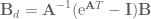
The cerebellum (CB) sub-network has two components to it: dynamics compensation and dynamics adaptation. First we’ll discuss the dynamics compensation. By which I mean the  term from the OSC signal.
Much like the calculating the kinematics term of the OSC signal in M1, we can calculate the entire dynamics compensation term using a single ensemble with an appropriate radius, scaled inputs, and well chosen intercepts.
def generate(arm, kv=1, learning_rate=None, learned_weights=None,
             means=None, scales=None):
    dim = arm.DOF * 2

    means = np.zeros(dim) if means is None else means
    scales = np.ones(dim) if scales is None else scales
    scale_down, scale_up = generate_scaling_functions(
        np.asarray(means), np.asarray(scales))

    net = nengo.Network('CB')
    with net:
        # create / connect up CB --------------------------------
        net.CB = nengo.Ensemble(
            n_neurons=1000, dimensions=dim,
            radius=np.sqrt(dim),
            intercepts=AreaIntercepts(
                dimensions=dim,
                base=nengo.dists.Uniform(-1, .1)))
        # expecting input in form [q, dq, u]
        net.input = nengo.Node(output=scale_down,
                               size_in=dim+arm.DOF+2)
        cb_input = nengo.Node(size_in=dim, label='CB input')
        nengo.Connection(net.input[:dim], cb_input)
        # output is [-Mdq, u_adapt]
        net.output = nengo.Node(size_in=arm.DOF*2)

        def CB_func(x):
            """ calculate the dynamic component of OSC signal """
            x = scale_up(x)
            q = x[:arm.DOF]
            dq = x[arm.DOF:arm.DOF*2]

            # calculate inertia matrix
            M = arm.M(q=q)
            return -np.dot(M, kv * dq)
        # connect up the input and output
        nengo.Connection(net.input[:dim], net.CB)
        nengo.Connection(net.CB, net.output[:arm.DOF],
                         function=CB_func, synapse=None)
I don’t think there’s anything noteworthy going on here, most of the relevant details have already been discussed…so we’ll move on to the adaptation!
Implementing CB – non-linear dynamics adaptation
The final part of the model is the non-linear dynamics adaptation, modelled as a separate ensemble in the cerebellar sub-network (a separate ensemble so that it’s more modular, the learning connection could also come off of the other CB population). I work through the details and proof of the learning rule in the paper, so I’m not going to discuss that here. But I will restate the learning rule here:

where  are the neural decoders,
  is the learning rate,
  is the neural activity of the ensemble, and is the joint space control signal sent to the arm. This is a basic delta learning rule, where the decoders of the active neurons are modified to push the decoded function in a direction that reduces the error.
The adaptive ensemble can be initialized either using saved weights (passed in with the learned_weights paramater) or as all zeros. It is important to note that setting decoders to all zeros means that does not mean having zero neural activity, so learning will not be affected by this initialization.
        # dynamics adaptation------------------------------------
        if learning_rate is not None:
            net.CB_adapt = nengo.Ensemble(
                n_neurons=1000, dimensions=arm.DOF*2,
                radius=np.sqrt(arm.DOF*2),
                # enforce spiking neurons
                neuron_type=nengo.LIF(),
                intercepts=AreaIntercepts(
                    dimensions=arm.DOF,
                    base=nengo.dists.Uniform(-.5, .2)))

            net.learn_encoders = nengo.Connection(
                net.input[:arm.DOF*2], net.CB_adapt,)

            # if no saved weights were passed in start from zero
            weights = (
                learned_weights if learned_weights is not None
                else np.zeros((arm.DOF, net.CB_adapt.n_neurons)))
            net.learn_conn = nengo.Connection(
                # connect directly to arm so that adaptive signal
                # is not included in the training signal
                net.CB_adapt.neurons, net.output[arm.DOF:],
                transform=weights,
                learning_rule_type=nengo.PES(
                    learning_rate=learning_rate),
                synapse=None)

            nengo.Connection(net.input[dim:dim+2],
                             net.learn_conn.learning_rule,
                             transform=-1, synapse=.01)
    return net
We’re able to implement that learning rule using Nengo’s prescribed error-sensitivity (PES) learning on our connection from the adaptive ensemble to the output. With this set up the system will be able to learn to adapt to perturbations that are functions of the input (set here to be ![[\textbf{q}, \dot{\textbf{q}}]](https://s0.wp.com/latex.php?latex=%5B%5Ctextbf%7Bq%7D%2C+%5Cdot%7B%5Ctextbf%7Bq%7D%7D%5D&bg=ffffff&fg=555555&s=0&c=20201002) ).
).
The intercepts in this population are set to values I found worked well for adapting to a few different forces, but it’s definitely a parameter to play with in your own scripts if you’re finding that there’s too much or not enough generalization of the decoded function output across the state space.
One other thing to mention is that we need to have a relay node to amalgamate the control signals output from M1 and the dynamics compensation ensemble in the CB. This signal is used to train the adaptive ensemble, and it’s important that the adaptive ensemble’s output is not included in the training signal, or else the system quickly goes off to positive or negative infinity.
Implementing S1 – a placeholder
The last sub-network in the REACH model is a placeholder for a primary sensory cortex (S1) model. This is just a set of ensembles that represents the feedback from the arm and relay it on to the rest of the model.
def generate(arm, direct_mode=False, means=None, scales=None):
    dim = arm.DOF*2 + 2  # represents [q, dq, hand_xy]

    means = np.zeros(dim) if means is None else means
    scales = np.ones(dim) if scales is None else scales
    scale_down, scale_up = generate_scaling_functions(
        np.asarray(means), np.asarray(scales))

    net = nengo.Network('S1')
    with net:
        # create / connect up S1 --------------------------------
        net.S1 = nengo.networks.EnsembleArray(
            n_neurons=50, n_ensembles=dim)

        # expecting input in form [q, x_des]
        net.input = nengo.Node(output=scale_down, size_in=dim)
        net.output = nengo.Node(
            lambda t, x: scale_up(x), size_in=dim)

        # send in system feedback and target information
        # don't account for synapses twice
        nengo.Connection(net.input, net.S1.input, synapse=None)
        nengo.Connection(net.S1.output, net.output, synapse=None)

    return net
Since there’s no function that we’re decoding off of the represented variables we can use separate ensembles to represent each dimension with an EnsembleArray. If we were going to decode some function of, for example, q0 and dq0, then we would need an ensemble that represents both variables. But since we’re just decoding out f(x) = x, using an EnsembleArray is a convenient way to decrease the number of neurons needed to accurately represent the input.
Creating a model using the framework
The REACH model has been set up to be as much of a plug and play system as possible. To generate a model you first create the M1, PMC, CB, and S1 networks, and then they’re all hooked up to each other using the framework.py file. Here’s an example script that controls the arm to trace a circle:
def generate():
    kp = 200
    kv = np.sqrt(kp) * 1.5

    center = np.array([0, 1.25])
    arm_sim = arm.Arm2Link(dt=1e-3)
    # set the initial position of the arm
    arm_sim.init_q = arm_sim.inv_kinematics(center)
    arm_sim.reset()

    net = nengo.Network(seed=0)
    with net:
        net.dim = arm_sim.DOF
        net.arm_node = arm_sim.create_nengo_node()
        net.error = nengo.Ensemble(1000, 2)
        net.xy = nengo.Node(size_in=2)

        # create an M1 model -------------------------------------
        net.M1 = M1.generate(arm_sim, kp=kp,
                             operational_space=True,
                             inertia_compensation=True,
                             means=[0.6, 2.2, 0, 0],
                             scales=[.5, .5, .25, .25])

        # create an S1 model -------------------------------------
        net.S1 = S1.generate(arm_sim,
                             means=[.6, 2.2, -.5, 0, 0, 1.25],
                             scales=[.5, .5, 1.7, 1.5, .75, .75])

        # subtract current position to get task space direction
        nengo.Connection(net.S1.output[net.dim*2:], net.error,
                         transform=-1)

        # create a trajectory for the hand to follow -------------
        x = np.linspace(0.0, 2.0*np.pi, 100)
        PMC_trajectory = np.vstack([np.cos(x) * .5,
                                    np.sin(x) * .5])
        PMC_trajectory += center[:, None]
        # create / connect up PMC --------------------------------
        net.PMC = PMC.generate(PMC_trajectory, speed=1)
        # send target for calculating control signal
        nengo.Connection(net.PMC.output, net.error)
        # send target (x,y) for plotting
        nengo.Connection(net.PMC.output, net.xy)

        net.CB = CB.generate(arm_sim, kv=kv,
                             means=[0.6, 2.2, -.5, 0],
                             scales=[.5, .5, 1.6, 1.5])

    model = framework.generate(net=net, probes_on=True)
    return model
In line 50 you can see the call to the framework code, which will hook up the most common connections that don’t vary between the different scripts.
The REACH model has assigned functionality to each area / sub-network, and you can see the expected input / output in the comments at the top of each sub-network file, but the implementations are open. You can create your own M1, PMC, CB, or S1 sub-networks and try them out in the context of a full model that generates high-level movement behaviour.
Running the model
To run the model you’ll need Nengo, Nengo GUI, and NengoLib all installed. You can then pull open Nengo GUI and load any of the a# scripts. In all of these scripts the S1 model is just an ensemble that represents the output from the arm_node. Here’s what each of the scripts does:
a01 has a spiking M1 and CB, dynamics adaptation turned off. The model guides the arm in reaching in a straight line to a single target and back.a02 has a spiking M1, PMC, and CB, dynamics adaptation turned off. The PMC generates a path for the hand to follow that traces out a circle.a03 has a spiking M1, PMC, and CB, dynamics adaptation turned off. The PMC generates a path for the joints to follow, which moves the hand in a straight line to a target and back.a04 has a spiking M1 and CB, dynamics adaptation turned off. The model performs the centre-out reaching task, starting at a central point and reaching to 8 points around a circle.a05 has a spiking M1 and CB, and dynamics adaptation turned on. The model performs the centre-out reaching task, starting at a central point and reaching to 8 points around a circle. As the model reaches, a forcefield is applied based on the joint velocities that pushes the arm as it tries to reach the target. After 100-150 seconds of simulation the arm has adapted and learned to reach in a straight line again.
Here’s what it looks like when you pull open a02 in Nengo GUI:

I’m not going to win any awards for arm animation, but! It’s still a useful visualization, and if anyone is proficient in javascript and want’s to improve it, please do! You can see the network architecture in the top left, the spikes generated by M1 and CB to the right of that, the arm in the bottom left, and the path traced out by the hand just to the right of that. On the top right you can see the a02 script code, and below that the Nengo console.
Conclusions
One of the most immediate extensions (aside from any sort of model of S1) that comes to mind here is implementing a more detailed cerebellar model, as there are several anatomically detailed models which have the same supervised learner functionality (for example (Yamazaki and Nagao, 2012)).
Hopefully people find this post and the code useful for their own work, or at least interesting! In the ideal scenario this would be a community project, where researchers add models of different brain areas and we end up with a large library of implementations to build larger models with in a Mr. Potato Head kind of fashion.
You can find all of the code up on my GitHub. And again, this code all should have been publicly available along with the publication. Hopefully the code proves useful! If you have any questions about it please don’t hesitate to make a comment here or contact me through email, and I’ll get back to you as soon as I can.
 ,
,  and
and  denote
  and
and  . It’s important to remember that
  is denoting a velocity, and not a position, as we work through things or it could take you a lot longer to understand than it otherwise might…
![\left[ \begin{array}{c} \dot{\textbf{x}} \\ \pmb{\omega} \end{array} \right] = \textbf{J}(\textbf{q}) \; \dot{\textbf{q}}](https://s0.wp.com/latex.php?latex=%5Cleft%5B+%5Cbegin%7Barray%7D%7Bc%7D+%5Cdot%7B%5Ctextbf%7Bx%7D%7D+%5C%5C+%5Cpmb%7B%5Comega%7D+%5Cend%7Barray%7D+%5Cright%5D+%3D+%5Ctextbf%7BJ%7D%28%5Ctextbf%7Bq%7D%29+%5C%3B+%5Cdot%7B%5Ctextbf%7Bq%7D%7D&bg=ffffff&fg=555555&s=0&c=20201002)
 position of the hand, the angular velocity dimensions are stripped out of the Jacobian so that it’s a 3 x n_joints matrix rather than a 6 x n_joints matrix. So the orientation of the end-effector is not controlled at all. When we did this, we didn’t need to worry or know anything about the form of the angular velocities.
 and
and  , we want to calculate the rotation quaternion
  that takes us from
 here, we negate either the scalar or vector part of the quaternion, but not both.


 is the rotation matrix for the end-effector, and
  is the vector part of the unit quaternion that can be extracted from the rotation matrix
  .
. ,
, and
and  are the scalar and vector part of the quaternion representation of
 is the rotation matrix representing the desired orientation and
 and
and  are the scalar and vector components of the quaternions representing the end-effector and target orientations, respectively, and
  is defined in (Nakanishi eq 73):
![\left[ \begin{array}{ccc} 0 & -\textbf{x}[2] & \textbf{x}[1] \\ \textbf{x}[2] & 0 & -\textbf{x}[0] \\ -\textbf{x}[1] & \textbf{x}[0] & 0 \end{array} \right]](https://s0.wp.com/latex.php?latex=%5Cleft%5B+%5Cbegin%7Barray%7D%7Bccc%7D+0+%26+-%5Ctextbf%7Bx%7D%5B2%5D+%26+%5Ctextbf%7Bx%7D%5B1%5D+%5C%5C+%5Ctextbf%7Bx%7D%5B2%5D+%26+0+%26+-%5Ctextbf%7Bx%7D%5B0%5D+%5C%5C+-%5Ctextbf%7Bx%7D%5B1%5D+%26+%5Ctextbf%7Bx%7D%5B0%5D+%26+0+%5Cend%7Barray%7D+%5Cright%5D&bg=ffffff&fg=555555&s=0&c=20201002)

 cannot be controlled. 2) The rank of the Jacobian determines how many DOF can be controlled at the same time.
 variables can be controlled, but
  cannot be controlled because their corresponding rows are all zeros. So 3 variables can potentially be controlled, but because the Jacobian is rank 2 only two variables can be controlled at a time. If you try to control more than 2 DOF at a time things are going to go poorly. Here are some animations of trying to control 3 DOF vs 2 DOF in a 2 joint arm:

 and
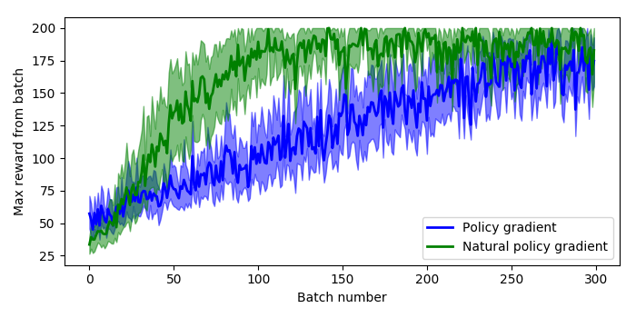
and  are the system state and chosen action at time
 are the network parameters that we’re learning
 is the control policy network parameterized
  is the advantage function, which returns the estimated total reward for taking action
 denotes calculating the partial derivative with respect to
  denotes that we’re using an estimation of the advantage function, and
  returns a scalar value which is the probability of the chosen action
  , which estimates the curvature of the control policy:
 . Including this then the weight update becomes
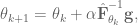

 that is normalized with respect to the change in the control policy. This is beneficial because it means that we don’t do any parameter updates that will drastically change the output of the policy network.

 for each
  pair along the trajectories sampled
 based on the sampled trajectories and the estimated value function
 as specified above

 was that the square root calculation was dying because negative values were being set in. This was very confusing because
  is a positive definite matrix, which means that
  is also positive definite, which means that
  for any
  .
.

 arm with joint torque sensors for the last year or so as part of our research at

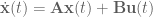
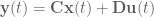
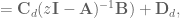
 is the system output,
 is called the input matrix,
 is called the output matrix, and
 is called the feedthrough matrix,
 is the Laplace variable.
 , giving:
 , such that
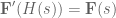
  has the same dynamics as our desired system,
  . In other words, find an
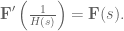

 , making our equation

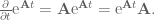
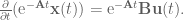
 . To do that, we can do the following basic math jujitsu


 . Said another way, we have created a system
 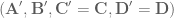 that compensates for the synaptic filtering effects to achieve our desired system dynamics!
 and
and  when implementing our model and we’re golden.
 instead of
  .
. . Rearranging things to put all the
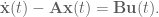
 (note the negative in the exponent)


 :
:


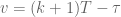
 for some time step
  , and that the input
  is constant between samples (this is where the ZOH comes in). To simplify our notation as we go, we also define
![\textbf{x}[k] = \textbf{x}(kT).](https://s0.wp.com/latex.php?latex=%5Ctextbf%7Bx%7D%5Bk%5D+%3D+%5Ctextbf%7Bx%7D%28kT%29.&bg=ffffff&fg=555555&s=0&c=20201002)
![\textbf{x}[k] = \textrm{e}^{\textbf{A}kT}\textbf{x}(0) + \textrm{e}^{\textbf{A}kT}\int_0^{kT} \textrm{e}^{-\textbf{A}\tau}\textbf{Bu}(\tau) d\tau.](https://s0.wp.com/latex.php?latex=%5Ctextbf%7Bx%7D%5Bk%5D+%3D+%5Ctextrm%7Be%7D%5E%7B%5Ctextbf%7BA%7DkT%7D%5Ctextbf%7Bx%7D%280%29+%2B+%5Ctextrm%7Be%7D%5E%7B%5Ctextbf%7BA%7DkT%7D%5Cint_0%5E%7BkT%7D+%5Ctextrm%7Be%7D%5E%7B-%5Ctextbf%7BA%7D%5Ctau%7D%5Ctextbf%7BBu%7D%28%5Ctau%29+d%5Ctau.&bg=ffffff&fg=555555&s=0&c=20201002)
![\textbf{x}[k+1] = \textbf{A}_d\textbf{x}[k] + \textbf{B}_d\textbf{u}[k].](https://s0.wp.com/latex.php?latex=%5Ctextbf%7Bx%7D%5Bk%2B1%5D+%3D+%5Ctextbf%7BA%7D_d%5Ctextbf%7Bx%7D%5Bk%5D+%2B+%5Ctextbf%7BB%7D_d%5Ctextbf%7Bu%7D%5Bk%5D.&bg=ffffff&fg=555555&s=0&c=20201002)
![\textbf{x}[k + 1]](https://s0.wp.com/latex.php?latex=%5Ctextbf%7Bx%7D%5Bk+%2B+1%5D&bg=ffffff&fg=555555&s=0&c=20201002)
![\textbf{x}[k+1] = \textrm{e}^{\textbf{A}(k+1)T}\textbf{x}(0) + \textrm{e}^{\textbf{A}(k+1)T}\int_0^{(k+1)T} \textrm{e}^{-\textbf{A}\tau}\textbf{Bu}(\tau) d\tau.](https://s0.wp.com/latex.php?latex=%5Ctextbf%7Bx%7D%5Bk%2B1%5D+%3D+%5Ctextrm%7Be%7D%5E%7B%5Ctextbf%7BA%7D%28k%2B1%29T%7D%5Ctextbf%7Bx%7D%280%29+%2B+%5Ctextrm%7Be%7D%5E%7B%5Ctextbf%7BA%7D%28k%2B1%29T%7D%5Cint_0%5E%7B%28k%2B1%29T%7D+%5Ctextrm%7Be%7D%5E%7B-%5Ctextbf%7BA%7D%5Ctau%7D%5Ctextbf%7BBu%7D%28%5Ctau%29+d%5Ctau.&bg=ffffff&fg=555555&s=0&c=20201002)
![\textbf{x}[k+1]](https://s0.wp.com/latex.php?latex=%5Ctextbf%7Bx%7D%5Bk%2B1%5D&bg=ffffff&fg=555555&s=0&c=20201002) to
to ![\textbf{x}[k]](https://s0.wp.com/latex.php?latex=%5Ctextbf%7Bx%7D%5Bk%5D&bg=ffffff&fg=555555&s=0&c=20201002) . Being incredibly clever, we see that we can left multiply
. Being incredibly clever, we see that we can left multiply  , to get
![\textrm{e}^{\textbf{A}T}\textbf{x}[k] = \textrm{e}^{\textbf{A}(k+1)T}\textbf{x}(0) + \textrm{e}^{\textbf{A}(k+1)T}\int_0^{kT} \textrm{e}^{-\textbf{A}\tau}\textbf{Bu}(\tau) d\tau,](https://s0.wp.com/latex.php?latex=%5Ctextrm%7Be%7D%5E%7B%5Ctextbf%7BA%7DT%7D%5Ctextbf%7Bx%7D%5Bk%5D+%3D+%5Ctextrm%7Be%7D%5E%7B%5Ctextbf%7BA%7D%28k%2B1%29T%7D%5Ctextbf%7Bx%7D%280%29+%2B+%5Ctextrm%7Be%7D%5E%7B%5Ctextbf%7BA%7D%28k%2B1%29T%7D%5Cint_0%5E%7BkT%7D+%5Ctextrm%7Be%7D%5E%7B-%5Ctextbf%7BA%7D%5Ctau%7D%5Ctextbf%7BBu%7D%28%5Ctau%29+d%5Ctau%2C&bg=ffffff&fg=555555&s=0&c=20201002)
![\textrm{e}^{\textbf{A}(k+1)T}\textbf{x}(0) = \textrm{e}^{\textbf{A}T}\textbf{x}[k] - \textrm{e}^{\textbf{A}(k+1)T}\int_0^{kT} \textrm{e}^{-\textbf{A}\tau}\textbf{Bu}(\tau) d\tau.](https://s0.wp.com/latex.php?latex=%5Ctextrm%7Be%7D%5E%7B%5Ctextbf%7BA%7D%28k%2B1%29T%7D%5Ctextbf%7Bx%7D%280%29+%3D+%5Ctextrm%7Be%7D%5E%7B%5Ctextbf%7BA%7DT%7D%5Ctextbf%7Bx%7D%5Bk%5D+-+%5Ctextrm%7Be%7D%5E%7B%5Ctextbf%7BA%7D%28k%2B1%29T%7D%5Cint_0%5E%7BkT%7D+%5Ctextrm%7Be%7D%5E%7B-%5Ctextbf%7BA%7D%5Ctau%7D%5Ctextbf%7BBu%7D%28%5Ctau%29+d%5Ctau.&bg=ffffff&fg=555555&s=0&c=20201002)
![\textbf{x}[k+1] = \textrm{e}^{\textbf{A}T}\textbf{x}[k] - \textrm{e}^{\textbf{A}(k+1)T}(\int_0^{kT} \textrm{e}^{-\textbf{A}\tau}\textbf{Bu}(\tau) d\tau + \int_0^{(k+1)T} \textrm{e}^{-\textbf{A}\tau}\textbf{Bu}(\tau) d\tau),](https://s0.wp.com/latex.php?latex=%5Ctextbf%7Bx%7D%5Bk%2B1%5D+%3D+%5Ctextrm%7Be%7D%5E%7B%5Ctextbf%7BA%7DT%7D%5Ctextbf%7Bx%7D%5Bk%5D+-+%5Ctextrm%7Be%7D%5E%7B%5Ctextbf%7BA%7D%28k%2B1%29T%7D%28%5Cint_0%5E%7BkT%7D+%5Ctextrm%7Be%7D%5E%7B-%5Ctextbf%7BA%7D%5Ctau%7D%5Ctextbf%7BBu%7D%28%5Ctau%29+d%5Ctau+%2B+%5Cint_0%5E%7B%28k%2B1%29T%7D+%5Ctextrm%7Be%7D%5E%7B-%5Ctextbf%7BA%7D%5Ctau%7D%5Ctextbf%7BBu%7D%28%5Ctau%29+d%5Ctau%29%2C&bg=ffffff&fg=555555&s=0&c=20201002)
![\textbf{x}[k+1] = \textrm{e}^{\textbf{A}T}\textbf{x}[k] - \textrm{e}^{\textbf{A}(k+1)T}\int_{kT}^{(k+1)T} \textrm{e}^{-\textbf{A}\tau}\textbf{Bu}(\tau) d\tau.](https://s0.wp.com/latex.php?latex=%5Ctextbf%7Bx%7D%5Bk%2B1%5D+%3D+%5Ctextrm%7Be%7D%5E%7B%5Ctextbf%7BA%7DT%7D%5Ctextbf%7Bx%7D%5Bk%5D+-+%5Ctextrm%7Be%7D%5E%7B%5Ctextbf%7BA%7D%28k%2B1%29T%7D%5Cint_%7BkT%7D%5E%7B%28k%2B1%29T%7D+%5Ctextrm%7Be%7D%5E%7B-%5Ctextbf%7BA%7D%5Ctau%7D%5Ctextbf%7BBu%7D%28%5Ctau%29+d%5Ctau.&bg=ffffff&fg=555555&s=0&c=20201002)
 is constant), we can take
  outside the integral.
![\textbf{x}[k+1] = \textrm{e}^{\textbf{A}T}\textbf{x}[k] - \textrm{e}^{\textbf{A}(k+1)T}\int_{kT}^{(k+1)T} \textrm{e}^{-\textbf{A}\tau}d\tau \textbf{Bu}[k].](https://s0.wp.com/latex.php?latex=%5Ctextbf%7Bx%7D%5Bk%2B1%5D+%3D+%5Ctextrm%7Be%7D%5E%7B%5Ctextbf%7BA%7DT%7D%5Ctextbf%7Bx%7D%5Bk%5D+-+%5Ctextrm%7Be%7D%5E%7B%5Ctextbf%7BA%7D%28k%2B1%29T%7D%5Cint_%7BkT%7D%5E%7B%28k%2B1%29T%7D+%5Ctextrm%7Be%7D%5E%7B-%5Ctextbf%7BA%7D%5Ctau%7Dd%5Ctau+%5Ctextbf%7BBu%7D%5Bk%5D.&bg=ffffff&fg=555555&s=0&c=20201002)
 term inside the integral:
![\textbf{x}[k+1] = \textrm{e}^{\textbf{A}T}\textbf{x}[k] - \int_{kT}^{(k+1)T} \textrm{e}^{\textbf{A}((k+1)T - \tau)}d\tau \textbf{Bu}[k].](https://s0.wp.com/latex.php?latex=%5Ctextbf%7Bx%7D%5Bk%2B1%5D+%3D+%5Ctextrm%7Be%7D%5E%7B%5Ctextbf%7BA%7DT%7D%5Ctextbf%7Bx%7D%5Bk%5D+-+%5Cint_%7BkT%7D%5E%7B%28k%2B1%29T%7D+%5Ctextrm%7Be%7D%5E%7B%5Ctextbf%7BA%7D%28%28k%2B1%29T+-+%5Ctau%29%7Dd%5Ctau+%5Ctextbf%7BBu%7D%5Bk%5D.&bg=ffffff&fg=555555&s=0&c=20201002)
 , which means also that
 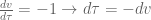 . Evaluating the upper and lower bounds of the integral, when
  then
then  and when
  then
then  . With this, we can rewrite our equation:
![\textbf{x}[k+1] = \textrm{e}^{\textbf{A}T}\textbf{x}[k] - \int_T^0 \textrm{e}^{\textbf{A}v}dv \textbf{Bu}[k].](https://s0.wp.com/latex.php?latex=%5Ctextbf%7Bx%7D%5Bk%2B1%5D+%3D+%5Ctextrm%7Be%7D%5E%7B%5Ctextbf%7BA%7DT%7D%5Ctextbf%7Bx%7D%5Bk%5D+-+%5Cint_T%5E0+%5Ctextrm%7Be%7D%5E%7B%5Ctextbf%7BA%7Dv%7Ddv+%5Ctextbf%7BBu%7D%5Bk%5D.&bg=ffffff&fg=555555&s=0&c=20201002)
 . We can just swap the bounds and multiply by
  , giving:
![\textbf{x}[k+1] = \textrm{e}^{\textbf{A}T}\textbf{x}[k] + \int_0^T \textrm{e}^{\textbf{A}v}dv \textbf{Bu}[k].](https://s0.wp.com/latex.php?latex=%5Ctextbf%7Bx%7D%5Bk%2B1%5D+%3D+%5Ctextrm%7Be%7D%5E%7B%5Ctextbf%7BA%7DT%7D%5Ctextbf%7Bx%7D%5Bk%5D+%2B+%5Cint_0%5ET+%5Ctextrm%7Be%7D%5E%7B%5Ctextbf%7BA%7Dv%7Ddv+%5Ctextbf%7BBu%7D%5Bk%5D.&bg=ffffff&fg=555555&s=0&c=20201002)
 and assuming that
 ![\textbf{x}[k+1] = \textrm{e}^{\textbf{A}T}\textbf{x}[k] + \textbf{A}^{-1} \textrm{e}^{\textbf{A}v}|^T_{v=0} \textbf{Bu}[k].](https://s0.wp.com/latex.php?latex=%5Ctextbf%7Bx%7D%5Bk%2B1%5D+%3D+%5Ctextrm%7Be%7D%5E%7B%5Ctextbf%7BA%7DT%7D%5Ctextbf%7Bx%7D%5Bk%5D+%2B+%5Ctextbf%7BA%7D%5E%7B-1%7D+%5Ctextrm%7Be%7D%5E%7B%5Ctextbf%7BA%7Dv%7D%7C%5ET_%7Bv%3D0%7D+%5Ctextbf%7BBu%7D%5Bk%5D.&bg=ffffff&fg=555555&s=0&c=20201002)
![\textbf{x}[k+1] = \textrm{e}^{\textbf{A}T}\textbf{x}[k] + \textbf{A}^{-1} (\textrm{e}^{\textbf{A}T} - \textrm{e}^0) \textbf{Bu}[k].](https://s0.wp.com/latex.php?latex=%5Ctextbf%7Bx%7D%5Bk%2B1%5D+%3D+%5Ctextrm%7Be%7D%5E%7B%5Ctextbf%7BA%7DT%7D%5Ctextbf%7Bx%7D%5Bk%5D+%2B+%5Ctextbf%7BA%7D%5E%7B-1%7D+%28%5Ctextrm%7Be%7D%5E%7B%5Ctextbf%7BA%7DT%7D+-+%5Ctextrm%7Be%7D%5E0%29+%5Ctextbf%7BBu%7D%5Bk%5D.&bg=ffffff&fg=555555&s=0&c=20201002)
![\textbf{x}[k+1] = \textrm{e}^{\textbf{A}T}\textbf{x}[k] + \textbf{A}^{-1} (\textrm{e}^{\textbf{A}T} - \textbf{I}) \textbf{Bu}[k].](https://s0.wp.com/latex.php?latex=%5Ctextbf%7Bx%7D%5Bk%2B1%5D+%3D+%5Ctextrm%7Be%7D%5E%7B%5Ctextbf%7BA%7DT%7D%5Ctextbf%7Bx%7D%5Bk%5D+%2B+%5Ctextbf%7BA%7D%5E%7B-1%7D+%28%5Ctextrm%7Be%7D%5E%7B%5Ctextbf%7BA%7DT%7D+-+%5Ctextbf%7BI%7D%29+%5Ctextbf%7BBu%7D%5Bk%5D.&bg=ffffff&fg=555555&s=0&c=20201002)


 and
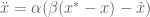
and  being the system position, velocity, and acceleration, respectively,
  is the target position, and
  and
and ![\left [ \begin{array}{c} \dot{x} \\ \ddot{x} \end{array} \right ] = \left [ \begin{array}{cc}0 & 1 \\ -\alpha\beta & -\alpha \end{array} \right] \left [ \begin{array}{c} x \\ \dot{x} \end{array} \right ] + \left [ \begin{array}{c}0 \\ \alpha\beta \end{array} \right] \left [ \begin{array}{c} 0 \\ x^* \end{array} \right ]](https://s0.wp.com/latex.php?latex=%5Cleft+%5B+%5Cbegin%7Barray%7D%7Bc%7D+%5Cdot%7Bx%7D+%5C%5C+%5Cddot%7Bx%7D+%5Cend%7Barray%7D+%5Cright+%5D+%3D+%5Cleft+%5B+%5Cbegin%7Barray%7D%7Bcc%7D0+%26+1+%5C%5C+-%5Calpha%5Cbeta+%26+-%5Calpha+%5Cend%7Barray%7D+%5Cright%5D+%5Cleft+%5B+%5Cbegin%7Barray%7D%7Bc%7D+x+%5C%5C+%5Cdot%7Bx%7D+%5Cend%7Barray%7D+%5Cright+%5D+%2B+%5Cleft+%5B+%5Cbegin%7Barray%7D%7Bc%7D0+%5C%5C+%5Calpha%5Cbeta+%5Cend%7Barray%7D+%5Cright%5D+%5Cleft+%5B+%5Cbegin%7Barray%7D%7Bc%7D+0+%5C%5C+x%5E%2A+%5Cend%7Barray%7D+%5Cright+%5D+&bg=ffffff&fg=555555&s=0&c=20201002)

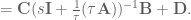
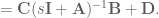
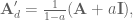
 , we’ll first calculate the discrete state matrices:

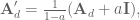

 .
.


