Robot control part 2: Jacobians, velocity, and force

Jacobian matrices are a super useful tool, and heavily used throughout robotics and control theory. Basically, a Jacobian defines the dynamic relationship between two different representations of a system. For example, if we have a 2-link robotic arm, there are two obvious ways to describe its current position: 1) the end-effector position and orientation (which we will denote $\textbf{x}$ ), and 2) as the set of joint angles (which we will denote $\textbf{q}$ ). The Jacobian for this system relates how movement of the elements of $\textbf{q}$ causes movement of the elements of $\textbf{x}$ . You can think of a Jacobian as a transform matrix for velocity.

Formally, a Jacobian is a set of partial differential equations:

$\textbf{J} = \frac{\partial \textbf{x}}{\partial \textbf{q}}$ .

With a bit of manipulation we can get a neat result:

$\textbf{J} = \frac{\partial \textbf{x}}{\partial t} \; \frac{\partial t}{\partial \textbf{q}} \rightarrow \frac{\partial \textbf{x}}{\partial \textbf{t}} = \textbf{J} \frac{\partial \textbf{q}}{\partial t}$ ,

$\dot{\textbf{x}} = \textbf{J} \; \dot{\textbf{q}}$ ,

where $\dot{\textbf{x}}$ and $\dot{\textbf{q}}$ represent the time derivatives of $\textbf{x}$ and $\textbf{q}$ . This tells us that the end-effector velocity is equal to the Jacobian, $\textbf{J}$ , multiplied by the joint angle velocity.

Why is this important? Well, this goes back to our desire to control in operational (or task) space. We’re interested in planning a trajectory in a different space than the one that we can control directly. Iin our robot arm, control is effected through a set of motors that apply torque to the joint angles, BUT what we’d like is to plan our trajectory in terms of end-effector position (and possibly orientation), generating control signals in terms of forces to apply in $(x,y,z)$ space. Jacobians allow us a direct way to calculate what the control signal is in the space that we control (torques), given a control signal in one we don’t (end-effector forces). The above equivalence is a first step along the path to operational space control. As just mentioned, though, what we’re really interested in isn’t relating velocities, but forces. How can we do this?

Energy equivalence and Jacobians
Conservation of energy is a property of all physical systems where the amount of energy expended is the same no matter how the system in question is being represented. The planar two-link robot arm shown below will be used for illustration.

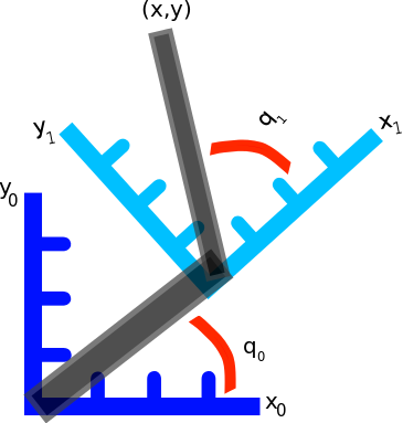
Let the joint angle positions be denoted $\textbf{q} = [q_0, q_1]^T$ , and end-effector position be denoted $\textbf{x} = [x, y, 0]^T$ .

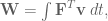
Work is the application of force over a distance

$\textbf{W} = \int \textbf{F}^T \textbf{v} \; dt,$

where $\textbf{W}$ is work, $\textbf{F}$ is force, and $\textbf{v}$ is velocity.

Power is the rate at which work is performed

$\textbf{P} = \frac{\textbf{W}}{t},$

where $\textbf{P}$ is power.
Substituting in the equation for work into the equation for power gives:

$\textbf{P} = \frac{\textbf{W}}{t} = \frac{\textbf{F}^T \textbf{d}}{t} = \textbf{F}^T \frac{\textbf{d}}{t} = \textbf{F}^T\textbf{v}.$

Because of energy equivalence, work is performed at the same rate regardless of the characterization of the system. Rewriting this terms of end-effector space gives:

$\textbf{P} = \textbf{F}_\textbf{x}^T \dot{\textbf{x}},$

where $\textbf{F}_\textbf{x}$ is the force applied to the hand, and $\dot{\textbf{x}}$ is the velocity of the hand. Rewriting the above in terms of joint-space gives:

$\textbf{P} = \textbf{F}_\textbf{q}^T \dot{\textbf{q}},$

where $\textbf{F}_\textbf{q}$ is the torque applied to the joints, and $\dot{\textbf{q}}$ is the angular velocity of the joints. Setting these two equations (in end-effector and joint space) equal to each other and substituting in our equation for the Jacobian gives:

$\textbf{F}_{q_{hand}}^T \dot{\textbf{q}} = \textbf{F}_\textbf{x}^T \dot{\textbf{x}},$

$\textbf{F}_{q_{hand}}^T \dot{\textbf{q}} = \textbf{F}_\textbf{x}^T \textbf{J}_{ee}(\textbf{q}) \; \dot{\textbf{q}},$

$\textbf{F}_{q_{hand}}^T \textbf{F}_\textbf{x}^T \textbf{J}_{ee}(\textbf{q}),$

$\textbf{F}_{q_{hand}} = \textbf{J}_{ee}^T(\textbf{q}) \textbf{F}_\textbf{x}.$

where $\textbf{J}_{ee}(\textbf{q})$ is the Jacobian for the end-effector of the robot, and $\textbf{F}_{q_{hand}}$ represents the forces in joint-space that affect movement of the hand. This says that not only does the Jacobian relate velocity from one state-space representation to another, it can also be used to calculate what the forces in joint space should be to effect a desired set of forces in end-effector space.

Building the Jacobian

First, we need to define the relationship between the $(x,y,z)$ position of the end-effector and the robot’s joint angles, $(q_0, q_1)$ . However will we do it? Well, we know the distances from the shoulder to the elbow, and elbow to the wrist, as well as the joint angles, and we’re interested in finding out where the end-effector is relative to a base coordinate frame…OH MAYBE we should use those forward transformation matrices from the previous post. Let’s do it!

The forward transformation matrix

Recall that transformation matrices allow a given point to be transformed between different reference frames. In this case, the position of the end-effector relative to the second joint of the robot arm is known, but where it is relative to the base reference frame (the first joint reference frame in this case) is of interest. This means that only one transformation matrix is needed, transforming from the reference frame attached to the second joint back to the base.

The rotation part of this matrix is straight-forward to define, as in the previous section:

$^1_0\textbf{R} = \left[ \begin{array}{ccc} cos(q_0) & -sin(q_0) & 0 \\ sin(q_0) & cos(q_0) & 0 \\ 0 & 0 & 1 \end{array} \right].$

The translation part of the transformation matrices is a little different than before because reference frame 1 changes as a function of the angle of the previous joint’s angles. From trigonometry, given a vector of length $r$ and an angle $q$ the $x$ position of the end point is defined $r \; cos(q)$ , and the $y$ position is $r \; sin(q)$ . The arm is operating in the $(x,y)$ plane, so the $z$ position will always be 0.

Using this knowledge, the translation part of the transformation matrix is defined:

$^1_0\textbf{D} = \left[ \begin{array}{c} L_0 cos(q_0) \\ L_0 sin(q_0) \\ 0 \end{array} \right].$

Giving the forward transformation matrix:

$^1_0\textbf{T} = \left[ \begin{array}{cc} ^1_0\textbf{R} & ^1_0\textbf{D} \\ \textbf{0} & \textbf{1} \end{array} \right] = \left[ \begin{array}{cccc} cos(q_0) & -sin(q_0) & 0 & L_0 cos(q_0) \\ sin(q_0) & cos(q_0) & 0 & L_0 sin(q_0)\\ 0 & 0 & 1 & 0 \\ 0 & 0 & 0 & 1 \end{array} \right],$

which transforms a point from reference frame 1 (elbow joint) to reference frame 0 (shoulder joint / base).

The point of interest is the end-effector which is defined in reference frame 1 as a function of joint angle, $q_1$ and the length of second arm segment, $L_1$ :

$\textbf{x} = \left[ \begin{array}{c} L_1 cos(q_1) \\ L_1 sin(q_1) \\ 0 \\ 1 \end{array} \right].$

To find the position of our end-effector in terms of the origin reference frame multiply the point $\textbf{x}$ by the transformation $^1_0\textbf{T}$ :

$^1_0\textbf{T} \; \textbf{x} = \left[ \begin{array}{cccc} cos(q_0) & -sin(q_0) & 0 & L_0 cos(q_0) \\ sin(q_0) & cos(q_0) & 0 & L_0 sin(q_0)\\ 0 & 0 & 1 & 0 \\ 0 & 0 & 0 & 1 \end{array} \right] \; \left[ \begin{array}{c} L_1 cos(q_1) \\ L_1 sin(q_1) \\ 0 \\ 1 \end{array} \right],$

$^1_0\textbf{T} \textbf{x} = \left[ \begin{array}{c} L_1 cos(q_0) cos(q_1) - L_1 sin(q_0) sin(q_1) + L_0 cos(q_0) \\ L_1 sin(q_0) cos(q_1) + L_1 cos(q_0) sin(q_1) + L_0 sin(q_0) \\ 0 \\ 1 \end{array} \right]$

where, by pulling out the $L_1$ term and using the trig identities

$cos(\alpha)cos(\beta) - sin(\alpha)sin(\beta) = cos(\alpha + \beta),$

and

$sin(\alpha)cos(\beta) + cos(\alpha)sin(\beta) = sin(\alpha + \beta),$

the position of our end-effector can be rewritten:

$\left[ \begin{array}{c} L_0 cos(q_0) + L_1 cos(q_0 + q_1) \\ L_0 sin(q_0) + L_1 sin(q_0 + q_1) \\ 0 \end{array} \right],$

which is the position of the end-effector in terms of joint angles. As mentioned above, however, both the position of the end-effector and its orientation are needed; the rotation of the end-effector relative to the base frame must also be defined.

Accounting for orientation

Fortunately, defining orientation is simple, especially for systems with only revolute and prismatic joints (spherical joints will not be considered here). With prismatic joints, which are linear and move in a single plane, the rotation introduced is 0. With revolute joints, the rotation of the end-effector in each axis is simply a sum of rotations of each joint in their respective axes of rotation.

In the example case, the joints are rotating around the $z$ axis, so the rotation part of our end-effector state is

$\left[ \begin{array}{c} \omega_x \\ \omega_y \\ \omega_z \end{array} \right] = \left[ \begin{array}{c} 0 \\ 0 \\ q_0 + q_1 \end{array} \right],$

where $\omega$ denotes angular rotation. If the first joint had been rotating in a different plane, e.g. in the $(x, z)$ plane around the $y$ axis instead, then the orientation would be

$\left[ \begin{array}{c} \omega_x \\ \omega_y \\ \omega_z \end{array} \right] = \left[ \begin{array}{c} 0 \\ q_0 \\ q_1 \end{array} \right].$

Partial differentiation

Once the position and orientation of the end-effector have been calculated, the partial derivative of these equations need to be calculated with respect to the elements of $\textbf{q}$ . For simplicity, the Jacobian will be broken up into two parts, $J_v$ and $J_\omega$ , representing the linear and angular velocity, respectively, of the end-effector.

The linear velocity part of our Jacobian is:

$\textbf{J}_v(\textbf{q}) = \left[ \begin{array}{cc} \frac{\partial x}{\partial q_0} & \frac{\partial x}{\partial q_1} \\ \frac{\partial y}{\partial q_0} & \frac{\partial y}{\partial q_1} \\ \frac{\partial z}{\partial q_0} & \frac{\partial z}{\partial q_1} \end{array} \right] = \left[ \begin{array}{cc} -L_0 sin(q_0) - L_1 sin(q_0 + q_1) & - L_1 sin(q_0 + q_1) \\ L_0 cos(q_0) + L_1 cos(q_0 + q_1) & L_1 cos(q_0 + q_1) \\ 0 & 0 \end{array} \right].$

The angular velocity part of our Jacobian is:

$\textbf{J}_\omega(\textbf{q}) = \left[ \begin{array}{cc} \frac{\partial \omega_x}{\partial q_0} & \frac{\partial \omega_x}{\partial q_1} \\ \frac{\partial \omega_y}{\partial q_0} & \frac{\partial \omega_y}{\partial q_1} \\ \frac{\partial \omega_z}{\partial q_0} & \frac{\partial \omega_z}{\partial q_1} \end{array} \right] = \left[ \begin{array}{cc} 0 & 0 \\ 0 & 0 \\ 1 & 1 \end{array} \right].$

The full Jacobian for the end-effector is then:

$\textbf{J}_{ee}(\textbf{q}) = \left[ \begin{array}{c} \textbf{J}_v(\textbf{q}) \\ \textbf{J}_\omega(\textbf{q}) \end{array} \right] = \left[ \begin{array}{cc} -L_0 sin(q_0) - L_1 sin(q_0 + q_1) & - L_1 sin(q_0 + q_1) \\ L_0 cos(q_0) + L_1 cos(q_0 + q_1) & L_1 cos(q_0 + q_1) \\ 0 & 0 \\ 0 & 0 \\ 0 & 0 \\ 1 & 1 \end{array} \right].$

Analyzing the Jacobian

Once the Jacobian is built, it can be analysed for insight about the relationship between $\dot{\textbf{x}}$ and $\dot{\textbf{q}}$ .

For example, there is a large block of zeros in the middle of the Jacobian defined above, along the row corresponding to linear velocity along the $z$ axis, and the rows corresponding to the angular velocity around the $x$ and $y$ axes. This means that the $z$ position, and rotations $\omega_x$ and $\omega_y$ are not controllable. This can be seen by going back to the first Jacobian equation:

$\dot{\textbf{x}} = \textbf{J}_{ee}(\textbf{q})\;\dot{\textbf{q}}.$

No matter what the values of $\dot{\textbf{q}}$ , it is impossible to affect $\omega_x$ , $\omega_y$ , or $z$ , because the corresponding rows during the above multiplication with the Jacobian are $\textbf{0}$ . These rows of zeros in the Jacobian are referred to as its `null space’. Because these variables can’t be controlled, they will be dropped from both $\textbf{F}_\textbf{x}$ and $\textbf{J}(\textbf{q})$ .

Looking at the variables that can be affected it can be seen that given any two of $x, y, \omega_z$ the third can be calculated because the robot only has 2 degrees of freedom (the shoulder and elbow). This means that only two of the end-effector variables can actually be controlled. In the situation of controlling a robot arm, it is most useful to control the $(x,y)$ coordinates, so $\omega_z$ will be dropped from the force vector and Jacobian.

After removing the redundant term, the force vector representing the controllable end-effector forces is

$\textbf{F}_\textbf{x} = \left[ \begin{array}{c}f_x \\ f_y\end{array} \right],$

where $f_x$ is force along the $x$ axis, $f_y$ is force along the $y$ axis, and the Jacobian is written

$\textbf{J}_{ee}(\textbf{q}) = \left[ \begin{array}{cc} -L_0 sin(q_0) - L_1 sin(q_0 + q_1) & - L_1 sin(q_0 + q_1) \\ L_0 cos(q_0) + L_1 cos(q_0 + q_1) & L_1 cos(q_0 + q_1) \end{array} \right].$

If instead $f_{\omega_z}$ , i.e. torque around the $z$ axis, were chosen as a controlled force then the force vector and Jacobian would be (assuming force along the $x$ axis was also chosen):

$\textbf{F}_\textbf{x} = \left[ \begin{array}{c} f_x \\ f_{\omega_z}\end{array} \right],$
$\textbf{J}_{ee}(\textbf{q}) = \left[ \begin{array}{cc} -L_0 sin(q_0) - L_1 sin(q_0 + q_1) & - L_1 sin(q_0 + q_1) \\ 1 & 1 \end{array} \right].$

But we’ll stick with control of the $x$ and $y$ forces instead, as it’s a little more straightforward.

Using the Jacobian

With our Jacobian, we can find out what different joint angle velocities will cause in terms of the end-effector linear and angular velocities, and we can also transform desired $(x,y)$ forces into $(\theta_0, \theta_1)$ torques. Let’s do a couple of examples. Note that in the former case we’ll be using the full Jacobian, while in the latter case we can use the simplified Jacobian specified just above.

Example 1

Given known joint angle velocities with arm configuration

$\textbf{q} = \left[ \begin{array}{c} \frac{\pi}{4} \\ \frac{3 \pi}{8} \end{array}\right] \;\;\;\; \dot{\textbf{q}} = \left[ \begin{array}{c} \frac{\pi}{10} \\ \frac{\pi}{10} \end{array} \right]$

and arm segment lengths $L_i = 1$ , the $(x,y)$ velocities of the end-effector can be calculated by substituting in the system state at the current time into the equation for the Jacobian:

$\dot{\textbf{x}} = \textbf{J}_{ee}(\textbf{q}) \; \dot{\textbf{q}},$

$\dot{\textbf{x}} = \left[ \begin{array}{cc} - sin(\frac{\pi}{4}) - sin(\frac{\pi}{4} + \frac{3\pi}{8}) & - sin(\frac{\pi}{4} + \frac{3\pi}{8}) \\ cos(\frac{\pi}{4}) + cos(\frac{\pi}{4} + \frac{3\pi}{8}) & cos(\frac{\pi}{4} + \frac{3\pi}{8}) \\ 0 & 0 \\ 0 & 0 \\ 0 & 0 \\ 1 & 1 \end{array} \right] \; \left[ \begin{array}{c} \frac{\pi}{10} \\ \frac{\pi}{10} \end{array} \right],$

$\dot{\textbf{x}} = \left[ -0.8026, -0.01830, 0, 0, 0, \frac{\pi}{5} \right]^T.$

And so the end-effector is linear velocity is $(-0.8026, -0.01830, 0)^T$ , with angular velocity is $(0, 0, \frac{\pi}{5})^T$ .

Example 2

Given the same system and configuration as in the previous example as well as a trajectory planned in $(x,y)$ space, the goal is to calculate the torques required to get the end-effector to move as desired. The controlled variables will be forces along the $x$ and $y$ axes, and so the reduced Jacobian from the previous section will be used. Let the desired $(x,y)$ forces be

$\textbf{F}_\textbf{x} = \left[ \begin{array}{c} 1 \\ 1 \end{array}\right],$

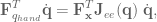
to calculate the corresponding joint torques the desired end-effector forces and current system state parameters are substituted into the equation relating forces in in end-effector and joint space:

$\textbf{F}_\textbf{q} = \textbf{J}^T_{ee}(\textbf{q}) \textbf{F}_\textbf{x},$

$\textbf{F}_\textbf{q} = \left[ \begin{array}{cc} -sin(\frac{\pi}{4}) -sin(\frac{\pi}{4} + \frac{3\pi}{8}) & cos(\frac{\pi}{4}) + cos(\frac{\pi}{4} + \frac{3\pi}{8}) \\ -sin(\frac{\pi}{4} + \frac{3\pi}{8}) & cos(\frac{\pi}{4} + \frac{3\pi}{8}) \end{array} \right] \left[ \begin{array}{c} 1 \\ 1 \end{array} \right],$

$\textbf{F}_\textbf{q} = \left[ \begin{array}{c} -1.3066 \\ -1.3066 \end{array}\right].$

So given the current configuration to get the end-effector to move as desired, without accounting for the effects of inertia and gravity, the torques to apply to the system are $\textbf{F}_\textbf{q} = [-1.3066, -1.3066]^T$ .

And now we are able to transform end-effector forces into torques, and joint angle velocities into end-effector velocities! What a wonderful, wonderful tool to have at our disposal! Hurrah for Jacobians!

Conclusions

In this post I’ve gone through how to use Jacobians to relate the movement of joint angle and end-effector system state characterizations, but Jacobians can be used to relate any two characterizations. All you need to do is define one in terms of the other and do some partial differentiation. The above example scenarios were of course very simple, and didn’t worry about compensating for anything like gravity. But don’t worry, that’s exactly what we’re going to look at in our exciting next chapter!

Something that I found interesting to consider is the need for the orientation of the end-effector and finding the angular velocities. Often in simpler robot arms, we’re only interested in the position of the end-effector, so it’s easy to write off orientation. But if we had a situation where there was a gripper attached to the end-effector, then suddenly the orientation becomes very important, often determining whether or not an object can be picked up or not.

And finally, if you’re interested in reading more about all this, I recommend checking out ‘Velocity kinematics – The manipulator Jacobian’ available online, it’s a great resource.

61 thoughts on “Robot control part 2: Jacobians, velocity, and force”

Robot control 3: Accounting for mass and gravity | studywolf says:

September 7, 2013 at 2:57 pm

[…] the exciting previous post we looked at how to go about generating a Jacobian matrix, which we could use to transformation […]

Robot control 4: Operation space control | studywolf says:

September 17, 2013 at 6:24 pm

[…] Once again, we’re going to need to find the Jacobians for the end-effector of the robot. Fortunately, we’ve already done this: […]

sc2013ironman says:

October 14, 2013 at 11:51 am

Reblogged this on Exoskeleton Project Blog.

CuPi says:

December 18, 2014 at 4:29 am

Thanks for your post
can you update the link which you recommend (book chapter online)

travisdewolf says:

December 18, 2014 at 9:10 am

can do! thanks for the notice that it was down!

Reply

Danylo says:

September 15, 2015 at 3:07 pm

What a great post! The second I saw your website, I knew I’ll be a frequent visitor. Thanks for the quality posts.

travisdewolf says:

September 15, 2015 at 3:16 pm

thank you very much for the kind words! glad you enjoy!

Reply

Bhardwaj Joshi says:

September 24, 2015 at 5:12 am

So wonderful explanation!! Thanks a lot, Travis

travisdewolf says:

September 24, 2015 at 8:26 am

Glad you found it useful! Thanks! 🙂

Reply

mrC says:

September 30, 2015 at 1:20 pm

Thank you for a good and informative article.
I have a question regarding the angular velocity jacobian, in the “Partial diffentiation” section. J_w(q) = dw/dq, so if you multiply this part of the jacobian with dq, would you not end up with dw, which is angular acceleration and not w?

travisdewolf says:

September 30, 2015 at 1:31 pm

Yup, dw = J_w(q)dq. I gave a quick scan for a typo but didn’t find it, is there a particular part that’s confusing?
Ah, is it in using J_w instead of J_alpha, where alpha represents angular velocity?

Reply
- mrC says:
  
  September 30, 2015 at 2:11 pm
  
  If I compare with the velocity jacobian, J_v(q)= dx/dq, then J_v*dq = dx = v, it ends up giving the velocity.
  But for the angular velocity jacobian,
  J_w(q)=dw/dq, here J_w(q)*dq = dw = alpha. It gives the angular acceleration, but J_w(q) should give angular velocity w?
- travisdewolf says:
  
  September 30, 2015 at 2:21 pm
  
  Ah, sorry it’s been a while since I wrote this and I forgot my own notation. So the Jacobian is defined between velocities, so the equation is not dw = J_w(q)*dq as I said in my last comment, but w = J_w(q)*dq, because w itself is d ang/dt, where ang is angular position .

Tharani says:

October 31, 2015 at 2:22 pm

Great explanation.

Juan Antonio says:

November 9, 2015 at 6:13 pm

Excellent information thanl you, I have a question , what happens if I want to find the jacobian between two point in the robot. For example I want to find the jacobian of a 5 DOFS biped robot (2 DOFS per leg and the Torso) between the foot o the robot and the COM (center of mass) how can I obtain the jacobian between this two parts. Could you help me?

thank you and regards.

travisdewolf says:

November 9, 2015 at 6:15 pm

Hi Juan,

thanks! You’ll need to measure each of the parts to find their lengths, and characterize the different rotations at each joint relative to each other. Doing this will give you the transformation matrix, once you have that you can take the derivative (by hand, or using sympy or mathematica) to give you the Jacobian. I go through another example here with a 6DOF arm which should hopefully help provide a template for you to follow: https://studywolf.wordpress.com/2015/06/27/operational-space-control-of-6dof-robot-arm-with-spiking-cameras-part-2-deriving-the-jacobian/
Good luck!

Reply
- Juan Antonio says:
  
  November 9, 2015 at 6:39 pm
  
  Thank you, I have a question, I need to find the transformation matrix only for the foot to the torso (3 DOFS) or I need to have the transformation matrix of all the system (5 DOFS)???
- travisdewolf says:
  
  November 9, 2015 at 9:03 pm
  
  You’ll need to have the transformation matrix for the whole system between the torso and foot, because movements of each of these joints will affect the force at the foot. Find the transformation matrix between each successive joint, and then multiply them together to get the transformation matrix for the whole system (from torso to foot).

sultan says:

December 9, 2015 at 5:57 pm

how can we avoid the singularity case

travisdewolf says:

December 9, 2015 at 6:02 pm

see exciting part 6! https://studywolf.wordpress.com/2013/10/10/robot-control-part-6-handling-singularities/

Reply

Jonathan Sebastian Obregon Flores says:

December 12, 2015 at 6:29 pm

Can you also find the position and orientation by finding the RPY angles of the rotational part from the homogeneous transformation matrix,then pulling the translational part from the transformation matrix, then store these three RPY angles and these three elements from translation part, in a 6×1 extended vector, is that the same too?, the jacobian Jee you computed is the analitical jacobian for the final effector, right?

travisdewolf says:

December 14, 2015 at 1:16 pm

Hi Jonathan,

I’m not sure I understand what you’re proposing; you could store the information in a 6×1 matrix, but then you’d have to extract and process it in a specific way, rather than just performing the matrix multiplications, to move from reference frame to reference frame. Another method is storing the information and doing rotation / translation is with dual quaternions if you’re looking for a more efficient representation! And yes, the Jee is the Jacobian for the end-effector. Hope that helps!

Reply
- Jonathan Sebastian Obregon Flores says:
  
  December 14, 2015 at 11:10 pm
  
  Thanks for your reply, well with the extended vector i meant the pose of the end effector, but in this case, are you using Jee to map dq to the twist? or to map to the pose derivative?
- travisdewolf says:
  
  December 16, 2015 at 12:06 pm
  
  Hi Jonathan,
  
  while Jacobians are defined by mapping joint angle velocities to end-effector velocities at the beginning of the post, we go on to use Jee to transform forces applied to the end-effector into joint torques.
wkc says:

February 26, 2016 at 4:06 pm

The answer is yes since RPY, or Euler angles for example, are quantities that can be differentiated. However the presentation given here is only applicable to special cases, such as the planar motion case, where angular velocity can be integrated. Except for the special cases angular velocity is not the derivative of any function so there is nothing to differentiate to get a matrix of partials. The well-known dynamicist Whittaker refers to non-existent quantities like this as quasi-coordinates.

Reply

Mohamed says:

December 28, 2015 at 12:25 am

Hi 🙂

Thanks a lot for your post. I’ve a question as this topic is new for me, what is the diff between Part1 & Part2. In other words between calculate X by knowing Q in case of forward dynamics & Jacobians.

travisdewolf says:

December 28, 2015 at 8:23 am

Hi Mohamed,

you can use forward transformation matrices to calculate the position of the end effector given the angles of the joints, and you can use the Jacobian to calculate both the velocity of the end-effector given the angular velocities of each of the joints, and the torques to apply to each of the joints given a desired end-effector force.
Hope that helps!

Reply

jeev says:

February 9, 2016 at 11:49 pm

Hi,

What is a null vector? How can we calculate a null vector for a given robot configuration?

travisdewolf says:

February 10, 2016 at 12:12 am

Addressed in exciting part 5!

Reply

Mike says:

March 12, 2016 at 3:27 pm

Hi, Great post! Better than most text books.

Got a doubt, in the section ‘Accounting for orientation’, you have mentioned [w_x, w_y, w_z] = [0,0, q0+q1]. where, q0 and q1 are joint positions right? But you have mentioned w as angular velocity. That part was not exactly clear. Could you please clarify?

travisdewolf says:

March 15, 2016 at 10:21 am

Hi Mike,

thanks for the catch! That should be ‘angular rotation’, and I’ll fix that now! It’s used in the part of the Jacobian that calculates angular velocity, like how the position information is used in the part of the Jacobian that calculates the linear velocity. Does that help?

Reply
- Mike says:
  
  March 15, 2016 at 10:47 am
  
  Hi Travis, yes that helps.

snowcrash says:

May 13, 2016 at 10:23 am

Hi Travis. Awesome blog. I seem to be having some issues with the moore penrose method for solving the Jacobian. I get some very erratic results when increasing the number of joints in the simulation. For example, it works well with 2 revolute joints, but fails horribly with 7 spherical joints. Have you experienced anything similar?

travisdewolf says:

May 13, 2016 at 11:05 am

Oof, how does it work with 2 spherical joints? Or one? I have only had experience enough with spherical joints to know I avoid them when possible!

Reply
- snowcrash says:
  
  May 13, 2016 at 11:51 am
  
  the two spherical direcly maps to 6 degrees for freedom, so 6×6 jacobi – which gets psuedoinversed well. Above that it falls to bits. Im just wondering if its my matrix math thats letting me down for the solve. eg. a fullpuvlu solve to determine the joint angles.
- travisdewolf says:
  
  May 13, 2016 at 12:03 pm
  
  Hmm, stepping back a second: why are you find the inverse of the Jacobian?

snowcrash says:

May 13, 2016 at 12:11 pm

im attempting to solve for an n sized system, the required joint angles. The transpose method works fine, but i want to be able to inject joint limits into this, so i want to solve the moore penrose version as well. eg ∆θ = J†~e.

travisdewolf says:

May 13, 2016 at 1:15 pm

Ahh, sorry I have no insights off hand that could be helpful. Please let me know what you find out though!

Reply

AgroQuad – Jalark says:

October 27, 2016 at 5:23 am

[…] In Robotics, the Jacobian Matrix is widely used to relate the ‘Joint’ rates to the linear and angular velocities of the ‘Tool’. For a Quadcopter, the Jacobian Matrix is used to relate angular velocities in the Body Frame to the Inertial Frame. For a brief explanation, follow: Jacobians, Velocity and Force […]

Correction says:

November 16, 2016 at 10:17 am

P ( Power) should be F^T V , there is no time derivative in the definition of P.

travisdewolf says:

November 16, 2016 at 10:47 am

oof! that’s a big typo, thanks for catching it!

Reply

Rhyban says:

November 22, 2016 at 5:18 am

Hi ! Your work is very useful. However I have a problem in the orientation part. You take a simple example of two joints. In this case, the angular angles are simple to calculate, but it is not always the case. Does it exist a method to calculate these angles with the rotation part of the transformation matrix ?

travisdewolf says:

March 10, 2017 at 2:11 pm

Hello! Sorry I’m not sure I understand your question, could you rephrase it for me, please?

Reply
- Rhyban says:
  
  March 17, 2017 at 8:55 am
  
  Is it possible to know the end-effector orientation only with the transformation matrix in a complex case ? (Admitting the last frame is on the end-effector)
- travisdewolf says:
  
  March 17, 2017 at 8:59 am
  
  Yup, the rotation part of the transformation matrix (i.e. T[0:3, 0:3]) specifies the orientation. Once you have it calculated you can use it to get Euler angles or the quaternion, whichever orientation format you want.

Nsitu Ugur says:

December 14, 2016 at 6:29 am

Omg! at last i understand what the jacobian is. Thanks for the really good explanation.

Olmo says:

March 4, 2017 at 9:45 pm

Hello and thanks for the sharing so much information! I have been thinking of planning movements in the operational space, say moving the robot from point A to B. If the planner only considers the geometrical path in the operational space, then I see a constant path speed, but joints speeds might be too high. Do you know if and how the joint dynamics can be taken into account (maybe through the Jacobian?) and reduce the path speed when necessary? I hope you understand what I mean. Thanks for your help!

travisdewolf says:

March 5, 2017 at 8:53 pm

Hello! It sounds like you’re looking for something like the velocity limiting I described here: https://studywolf.wordpress.com/2016/11/07/velocity-limiting-in-operational-space-control/

It limits the velocity of the end-effector in operational space, which in turn can prevent the controller specifying torques the motors can’t match. It will require a bit of playing around with to find the right limits but I think it’s what you’re looking for!

Reply

Arda Putra Ryandika says:

March 25, 2017 at 9:00 pm

Thanks for the explanation, it helps a lot!

Anyway, I have a question. You didn’t create another homogenous transformation matrix for the last link, instead, you applied it as an end effector position. In my case, Until the end point, I kept using homogenous transformation so that it becomes two frame matrix :

Frame 0->1 and Frame 1->2 but I didn’t use L cos and L sin as my end effector points (x matrices)

I thought the result would turn out the same nonetheless, but when I applied it to different system it becomes different.

It might be my error in calculating the Jacobian, but what’s your thought in this matter?

travisdewolf says:

March 30, 2017 at 4:00 pm

Hi Arda,

hmmm yup those should be the same, unfortunately I think you might have an error in your calculations!
As I understand it you’ve got something like T01 * T12 * x, where x = [0, 0], rather than T01 * x with x = [l1*cos(q1), l1*sin(q1)]?
In both cases you should end up with equivalent expressions.
Good luck!

Reply

Sharmila Kayastha says:

March 28, 2017 at 10:23 pm

Hi, this is a very useful topic for me. It helps me to understand how to get the angular velocity of the end effector. Now, I want to calculate end effector angular acceleration. So, can we get it simply by taking derivative of the angular velocity of end effector? Or we need to do some other calculation?

travisdewolf says:

March 30, 2017 at 4:19 pm

Hi Sharmila, yup you can calculate it by taking the derivative of $\dot{\textbf{x}} = \textbf{J}\dot{\textbf{q}}$ , which works out to $\ddot{\textbf{x}} = \dot{\textbf{J}}\dot{\textbf{q}} + \textbf{J}\ddot{\textbf{q}}$ . They discuss computing $\dot{\textbf{J}}$ here. Essentially, to get dJ[i, j] you take J[i, j] and differentiate with respect to each joint, then sum all the results. Hope that helps!

Reply
- Sharmila Kayastha says:
  
  March 30, 2017 at 4:31 pm
  
  Thank you very much.

magdy says:

July 12, 2017 at 6:11 am

can you find modelling by three link robot manipulator (articulated)
forward dynamic -inverse dynamic -Jacobin- dynamic equation)

travisdewolf says:

August 28, 2017 at 3:29 pm

Hello, I’m afraid I don’t understand your question. Could you rephrase it for me?

Reply

Achyut Paudel says:

November 21, 2018 at 7:12 pm

I wanted to control my end effector position without doing the inverse kinematics and controling the force using a PD controller. How do I do that? I have a 3link arm and would like the last link to be horizontal while moving vertically.

travisdewolf says:

November 27, 2018 at 4:49 pm

Hi Achyut, do you mean controlling the orientation of the end effector as well as the position? I’m actually just in the middle of writing up a blog post about this, I hope to have it out in the next couple weeks. It’s unfortunately a bit too much for me to try to explain here, but if you’re in a rush about this you can email me too. Cheers,

Reply

Force control of task-space orientation | studywolf says:

December 3, 2018 at 4:38 pm

[…] if you recall a post long ago on Jacobians, our task-space Jacobian has 6 […]

Aaron says:

February 10, 2019 at 11:13 pm

Right now I am doing force control and have read your excellent blog. I have a question. Do you think the mass inertia matrix is important? Because I think the force feedback controller should be PD controller+ M(d^2(theta)/dt^2). If you have time, want to discuss with you in email. Thanks in advance! Right now I am using Solidworks Analysis for inertia matrix.
My payload is about 2kg in the end effector and the whole weight of 7 axis robot arm is about 8kg without any other sensors. The length is about 70cm.

travisdewolf says:

May 9, 2019 at 4:16 pm

Hi Aaron, the inertia matrix is definitely important. I’m not sure I understand your suggestion. Happy to chat with you over email, I’ll try to find it in my inbox.
Cheers,

Reply

Ryan says:

September 26, 2019 at 12:45 pm

Could anyone explain where the superscript “T” for matrix transpose comes in for the force/torque relations? I didn’t understand why they transpose was necessary in the derivations.

studywolf

a blog for things I encounter while coding and researching neuroscience, motor control, and learning