A few months ago I posted on Linear Quadratic Regulators (LQRs) for control of non-linear systems using finite-differences. The gist of it was at every time step linearize the dynamics, quadratize (it could be a word) the cost function around the current point in state space and compute your feedback gain off of that, as though the dynamics were both linear and consistent (i.e. didn’t change in different states). And that was pretty cool because you didn’t need all the equations of motion and inertia matrices etc to generate a control signal. You could just use the simulation you had, sample it a bunch to estimate the dynamics and value function, and go off of that.
The LQR, however, operates with maverick disregard for changes in the future. Careless of the consequences, it optimizes assuming the linear dynamics approximated at the current time step hold for all time. It would be really great to have an algorithm that was able to plan out and optimize a sequence, mindful of the changing dynamics of the system.
This is exactly the iterative Linear Quadratic Regulator method (iLQR) was designed for. iLQR is an extension of LQR control, and the idea here is basically to optimize a whole control sequence rather than just the control signal for the current point in time. The basic flow of the algorithm is:
- Initialize with initial state
 and initial control sequence
 ![\textbf{U} = [u_{t_0}, u_{t_1}, ..., u_{t_{N-1}}]](https://s0.wp.com/latex.php?latex=%5Ctextbf%7BU%7D+%3D+%5Bu_%7Bt_0%7D%2C+u_%7Bt_1%7D%2C+...%2C+u_%7Bt_%7BN-1%7D%7D%5D&bg=ffffff&fg=555555&s=0&c=20201002) .
.
- Do a forward pass, i.e. simulate the system using
 to get the trajectory through state space,
  , that results from applying the control sequence
  starting in .
- Do a backward pass, estimate the value function and dynamics for each
 in the state-space and control signal trajectories.
- Calculate an updated control signal
 and evaluate cost of trajectory resulting from
  .
.
- If
 then we've converged and exit.
- If
 , then set
  , and change the update size to be more aggressive. Go back to step 2.
- If

 change the update size to be more modest. Go back to step 3.
There are a bunch of descriptions of iLQR, and it also goes by names like ‘the sequential linear quadratic algorithm’. The paper that I’m going to be working off of is by Yuval Tassa out of Emo Todorov’s lab, called Control-limited differential dynamic programming. And the Python implementation of this can be found up on my github in my Control repo. Also, a big thank you to Dr. Emo Todorov who provided Matlab code for the iLQG algorithm, which was super helpful.
Defining things
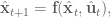
So let’s dive in. Formally defining things, we have our system  , and dynamics described with the function
  , such that

where  is the input control signal. The trajectory
  is the sequence of states
  that result from applying the control sequence
  starting in the initial state
  .
.
Now we need to define all of our cost related equations, so we know exactly what we’re dealing with.
Define the total cost function  , which is the sum of the immediate cost,
  , from each state in the trajectory plus the final cost,
  :
:
Letting  , we define the cost-to-go as the sum of costs from time
  to
to  :
:

The value function  at time is the optimal cost-to-go from a given state:

where the above equation just says that the optimal cost-to-go is found by using the control sequence  that minimizes
  .
.
At the final time step, , the value function is simply
For all preceding time steps, we can write the value function as a function of the immediate cost  and the value function at the next time step:
![V(\textbf{x}) = \min\limits_{\textbf{u}} \left[ \ell(\textbf{x}, \textbf{u}) + V(\textbf{f}(\textbf{x}, \textbf{u})) \right].](https://s0.wp.com/latex.php?latex=V%28%5Ctextbf%7Bx%7D%29+%3D+%5Cmin%5Climits_%7B%5Ctextbf%7Bu%7D%7D+%5Cleft%5B+%5Cell%28%5Ctextbf%7Bx%7D%2C+%5Ctextbf%7Bu%7D%29+%2B+V%28%5Ctextbf%7Bf%7D%28%5Ctextbf%7Bx%7D%2C+%5Ctextbf%7Bu%7D%29%29+%5Cright%5D.&bg=ffffff&fg=555555&s=0&c=20201002)
NOTE: In the paper, they use the notation  to denote the value function at the next time step, which is redundant since
  , but it comes in handy later when they drop the dependencies to simplify notation. So, heads up:
  .
.
Forward rollout
The forward rollout consists of two parts. The first part is to simulating things to generate the  from which we can calculate the overall cost of the trajectory, and find out the path that the arm will take. To improve things though we’ll need a lot of information about the partial derivatives of the system, calculating these is the second part of the forward rollout phase.
To calculate all these partial derivatives we’ll use  . For each
  we’ll calculate the derivatives of
  with respect to
  and
and  , which will give us what we need for our linear approximation of the system dynamics.
To get the information we need about the value function, we’ll need the first and second derivatives of  and
and  with respect to and .
So all in all, we need to calculate  ,
,  ,
,  ,
,  ,
,  ,
,  ,
,  , where the subscripts denote a partial derivative, so is the partial derivative of with respect to , is the second derivative of with respect to , etc. And to calculate all of these partial derivatives, we’re going to use finite differences! Just like in the LQR with finite differences post. Long story short, load up the simulation for every time step, slightly vary one of the parameters, and measure the resulting change.
Once we have all of these, we’re ready to move on to the backward pass.
Backward pass
Now, we started out with an initial trajectory, but that was just a guess. We want our algorithm to take it and then converge to a local minimum. To do this, we’re going to add some perturbing values and use them to minimize the value function. Specifically, we’re going to compute a local solution to our value function using a quadratic Taylor expansion. So let’s define  to be the change in our value function at as a result of small perturbations
  :
:

The second-order expansion of  is given by:


Remember that  , which is the value function at the next time step. NOTE: All of the second derivatives of are zero in the systems we’re controlling here, so when we calculate the second derivatives we don’t need to worry about doing any tensor math, yay!
Given the second-order expansion of , we can to compute the optimal modification to the control signal,  . This control signal update has two parts, a feedforward term,
  , and a feedback term
  . The optimal update is the
  that minimizes the cost of :

where  and
and 
Derivation can be found in this earlier paper by Li and Todorov. By then substituting this policy into the expansion of we get a quadratic model of . They do some mathamagics and come out with:

So now we have all of the terms that we need, and they’re defined in terms of the values at the next time step. We know the value of the value function at the final time step  , and so we’ll simply plug this value in and work backwards in time recursively computing the partial derivatives of and .
Calculate control signal update
Once those are all calculated, we can calculate the gain matrices, and  , for our control signal update. Huzzah! Now all that’s left to do is evaluate this new trajectory. So we set up our system


and record the cost. Now if the cost of the new trajectory  is less than the cost of then we set and go do it all again! And when the cost from an update becomes less than a threshold value, call it done. In code this looks like:
if costnew < cost:
  sim_new_trajectory = True

  if (abs(costnew - cost)/cost) < self.converge_thresh:
    break
Of course, another option we need to account for is when costnew > cost. What do we do in this case? Our control update hasn’t worked, do we just exit?
The Levenberg-Marquardt heuristic
No! Phew.
The control signal update in iLQR is calculated in such a way that it can behave like Gauss-Newton optimization (which uses second-order derivative information) or like gradient descent (which only uses first-order derivative information). The is that if the updates are going well, then lets include curvature information in our update to help optimize things faster. If the updates aren’t going well let’s dial back towards gradient descent, stick to first-order derivative information and use smaller steps. This wizardry is known as the Levenberg-Marquardt heuristic. So how does it work?
Something we skimmed over in the iLQR description was that we need to calculate  to get the and matrices. Instead of using
 np.linalg.pinv or somesuch, we’re going to calculate the inverse ourselves after finding the eigenvalues and eigenvectors, so that we can regularize it. This will let us do a couple of things. First, we’ll be able to make sure that our estimate of curvature ( ) stays positive definite, which is important to make sure that we always have a descent direction. Second, we’re going to add a regularization term to the eigenvalues to prevent them from exploding when we take their inverse. Here’s our regularization implemented in Python:
Q_uu_evals, Q_uu_evecs = np.linalg.eig(Q_uu)
Q_uu_evals[Q_uu_evals < 0] = 0.0
Q_uu_evals += lamb
Q_uu_inv = np.dot(Q_uu_evecs,
    np.dot(np.diag(1.0/Q_uu_evals), Q_uu_evecs.T))
Now, what happens when we change lamb? The eigenvalues represent the magnitude of each of the eigenvectors, and by taking their reciprocal we flip the contributions of the vectors. So the ones that were contributing the least now have the largest singular values, and the ones that contributed the most now have the smallest eigenvalues. By adding a regularization term we ensure that the inverted eigenvalues can never be larger than 1/lamb. So essentially we throw out information.
In the case where we’ve got a really good approximation of the system dynamics and value function, we don’t want to do this. We want to use all of the information available because it’s accurate, so make lamb small and get a more accurate inverse. In the case where we have a bad approximation of the dynamics we want to be more conservative, which means not having those large singular values. Smaller singular values give a smaller estimate, which then gives smaller gain matrices and control signal update, which is what we want to do when our control signal updates are going poorly.
How do you know if they’re going poorly or not, you now surely ask! Clever as always, we’re going to use the result of the previous iteration to update lamb. So adding to the code from just above, the end of our control update loop is going to look like:
lamb = 1.0 # initial value of lambda
...
if costnew < cost:
  lamb /= self.lamb_factor
  sim_new_trajectory = True

  if (abs(costnew - cost)/cost) < self.converge_thresh:
    break
else:
  lamb *= self.lamb_factor
  if lamb > self.max_lamb:
    break
And that is pretty much everything! OK let’s see how this runs!
Simulation results
If you want to run this and see for yourself, you can go copy my Control repo, navigate to the main directory, and run
python run.py arm2 reach
or substitute in arm3. If you’re having trouble getting the arm2 simulation to run, try arm2_python, which is a straight Python implementation of the arm dynamics, and should work no sweat for Windows and Mac.
Below you can see results from the iLQR controller controlling the 2 and 3 link arms (click on the figures to see full sized versions, they got distorted a bit in the shrinking to fit on the page), using immediate and final state cost functions defined as:
l = np.sum(u**2)
and
pos_err = np.array([self.arm.x[0] - self.target[0],
                    self.arm.x[1] - self.target[1]])
l = (wp * np.sum(pos_err**2) + # pos error
    wv * np.sum(x[self.arm.DOF:self.arm.DOF*2]**2)) # vel error
where wp and wv are just gain values, x is the state of the system, and self.arm.x is the  position of the hand. These read as “during movement, penalize large control signals, and at the final state, have a big penalty on not being at the target.”
So let’s give it up for iLQR, this is awesome! How much of a crazy improvement is that over LQR? And with all knowledge of the system through finite differences, and with the full movements in exactly 1 second! (Note: The simulation speeds look different because of my editing to keep the gif sizes small, they both take the same amount of time for each movement.)
Changing cost functions
Something that you may notice is that the control of the 3 link is actually straighter than the 2 link. I thought that this might be just an issue with the gain values, since the scale of movement is smaller for the 2 link arm than the 3 link there might have been less of a penalty for not moving in a straight line, BUT this was wrong. You can crank the gains and still get the same movement. The actual reason is that this is what the cost function specifies, if you look in the code, only  penalizes the distance from the target, and the cost function during movement is strictly to minimize the control signal, i.e.
  .
.
Well that’s a lot of talk, you say, like the incorrigible antagonist we both know you to be, prove it. Alright, fine! Here’s iLQR running with an updated cost function that includes the end-effector’s distance from the target in the immediate cost:

All that I had to do to get this was change the immediate cost from
l = np.sum(u**2)
to
l = np.sum(u**2)
pos_err = np.array([self.arm.x[0] - self.target[0],
                    self.arm.x[1] - self.target[1]])
l += (wp * np.sum(pos_err**2) + # pos error
    wv * np.sum(x[self.arm.DOF:self.arm.DOF*2]**2)) # vel error
where all I had to do was include the position penalty term from the final state cost into the immediate state cost.
Changing sequence length
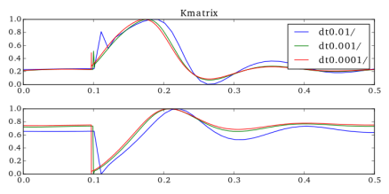
In these simulations the system is simulating at .01 time step, and I gave it 100 time steps to reach the target. What if I give it only 50 time steps?
It looks pretty much the same! It’s just now twice as fast, which is of course achieved by using larger control signals, which we don’t see, but dang awesome.
What if we try to make it there in 10 time steps??
OK well that does not look good. So what’s going on in this case? Basically we’ve given the algorithm an impossible task. It can’t make it to the target location in 10 time steps. In the implementation I wrote here, if it hits the end of it’s control sequence and it hasn’t reached the target yet, the control sequence starts over back at
t=0. Remember that part of the target state is also velocity, so basically it moves for 10 time steps to try to minimize
distance, and then slows down to minimize final state cost in the velocity term.
In conclusion
This algorithm has been used in a ton of things, for controlling robots and simulations, and is an important part of guided policy search, which has been used to very successfully train deep networks in control problems. It’s getting really impressive results for controlling the arm models that I’ve built here, and using finite differences should easily generalize to other systems.
iLQR is very computationally expensive, though, so that’s definitely a downside. It’s definitely less expensive if you have the equations of your system, or at least a decent approximation of them, and you don’t need to use finite differences. But you pay for the efficiency with a loss in generality.
There are also a bunch of parameters to play around with that I haven’t explored at all here, like the weights in the cost function penalizing the magnitude of the cost function and the final state position error. I showed a basic example of changing the cost function, which hopefully gets across just how easy changing these things out can be when you’re using finite differences, and there’s a lot to play around with there too.
Implementation note
In the Yuval and Todorov paper, they talked about using backtracking line search when generating the control signal. So the algorithm they had when generating the new control signal was actually:

where  was the backtracking search parameter, which gets set to one initially and then reduced. It’s very possible I didn’t implement it as intended, but I found consistently that
  always generated the best results, so it was just adding computation time. So I left it out of my implementation. If anyone has insights on an implementation that improves results, please let me know!
And then finally, another thank you to Dr. Emo Todorov for providing Matlab code for the iLQG algorithm, which was very helpful, especially for getting the Levenberg-Marquardt heuristic implemented properly.

 and
and  are gain terms,
  is the goal state,
  is the system state,
  is the system velocity, and
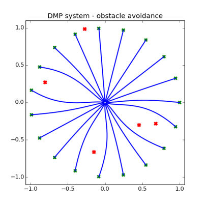
 implements the obstacle avoidance dynamics, and is a function of the DMP state and velocity. Now then, the question is what are these dynamics exactly?
 , here’s a picture of it:
 , as in the figure below:

 and
and  are constants, which are specified as
  and
and  in the paper, respectively.
 vector to get the cosine of the angle, and then use
 is the axis
  rotated 90 degrees (the
  denoting outer product here). The way I’ve been thinking about this is basically taking your velocity vector,
  axis, and the bottom row by the difference along the
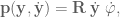
 instead of


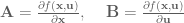
 ,
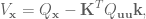
, are the state and its time derivative,
  and
and  capture the effects of the state and input on the derivative. And second, it assumes that the cost function, denoted
 is the target state, and
  and
and  are weights on the cost of not being at the target state and applying a control signal. The higher
  is, the more important it is to get to the target state asap, the higher

 ,
, .
. at the point
  . Here’s a picture for a 1D system:
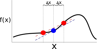
 and
and  . We can then calculate
 ,
,
 . If you’re solving for
  . This was just something that I came across as I was coding and so I wanted to mention it here in case anyone else stumbled across it!


 ). The Jacobian for this system relates how movement of the elements of
  .
. ,
, ,
, represent the time derivatives of
  , multiplied by the joint angle velocity.
 space. Jacobians allow us a direct way to calculate what the control signal is in the space that we control (torques), given a control signal in one we don’t (end-effector forces). The above equivalence is a first step along the path to operational space control. As just mentioned, though, what we’re really interested in isn’t relating velocities, but forces. How can we do this?
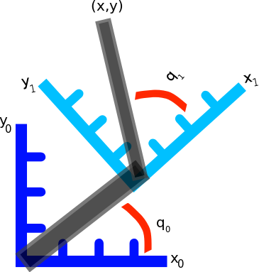
![\textbf{q} = [q_0, q_1]^T](https://s0.wp.com/latex.php?latex=%5Ctextbf%7Bq%7D+%3D+%5Bq_0%2C+q_1%5D%5ET&bg=ffffff&fg=555555&s=0&c=20201002) , and end-effector position be denoted
, and end-effector position be denoted ![\textbf{x} = [x, y, 0]^T](https://s0.wp.com/latex.php?latex=%5Ctextbf%7Bx%7D+%3D+%5Bx%2C+y%2C+0%5D%5ET&bg=ffffff&fg=555555&s=0&c=20201002) .
.
 is work,
  is force, and
  is velocity.
 is power.

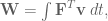
 is the force applied to the hand, and
 is the torque applied to the joints, and
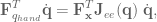


 is the Jacobian for the end-effector of the robot, and
  represents the forces in joint-space that affect movement of the hand. This says that not only does the Jacobian relate velocity from one state-space representation to another, it can also be used to calculate what the forces in joint space should be to effect a desired set of forces in end-effector space.
 . However will we do it? Well, we know the distances from the shoulder to the elbow, and elbow to the wrist, as well as the joint angles, and we’re interested in finding out where the end-effector is relative to a base coordinate frame…OH MAYBE we should use those forward transformation matrices from the previous post. Let’s do it!
![^1_0\textbf{R} = \left[ \begin{array}{ccc} cos(q_0) & -sin(q_0) & 0 \\ sin(q_0) & cos(q_0) & 0 \\ 0 & 0 & 1 \end{array} \right].](https://s0.wp.com/latex.php?latex=%5E1_0%5Ctextbf%7BR%7D+%3D+%5Cleft%5B+%5Cbegin%7Barray%7D%7Bccc%7D+cos%28q_0%29+%26+-sin%28q_0%29+%26+0+%5C%5C+sin%28q_0%29+%26+cos%28q_0%29+%26+0+%5C%5C+0+%26+0+%26+1+%5Cend%7Barray%7D+%5Cright%5D.&bg=ffffff&fg=555555&s=0&c=20201002)
 and an angle
  the
the  , and the
  position is
  . The arm is operating in the
  position will always be 0.
![^1_0\textbf{D} = \left[ \begin{array}{c} L_0 cos(q_0) \\ L_0 sin(q_0) \\ 0 \end{array} \right].](https://s0.wp.com/latex.php?latex=%5E1_0%5Ctextbf%7BD%7D+%3D+%5Cleft%5B+%5Cbegin%7Barray%7D%7Bc%7D+L_0+cos%28q_0%29+%5C%5C+L_0+sin%28q_0%29+%5C%5C+0+%5Cend%7Barray%7D+%5Cright%5D.+&bg=ffffff&fg=555555&s=0&c=20201002)
![^1_0\textbf{T} = \left[ \begin{array}{cc} ^1_0\textbf{R} & ^1_0\textbf{D} \\ \textbf{0} & \textbf{1} \end{array} \right] = \left[ \begin{array}{cccc} cos(q_0) & -sin(q_0) & 0 & L_0 cos(q_0) \\ sin(q_0) & cos(q_0) & 0 & L_0 sin(q_0)\\ 0 & 0 & 1 & 0 \\ 0 & 0 & 0 & 1 \end{array} \right],](https://s0.wp.com/latex.php?latex=%5E1_0%5Ctextbf%7BT%7D+%3D+%5Cleft%5B+%5Cbegin%7Barray%7D%7Bcc%7D+%5E1_0%5Ctextbf%7BR%7D+%26+%5E1_0%5Ctextbf%7BD%7D+%5C%5C+%5Ctextbf%7B0%7D+%26+%5Ctextbf%7B1%7D+%5Cend%7Barray%7D+%5Cright%5D+%3D+%5Cleft%5B+%5Cbegin%7Barray%7D%7Bcccc%7D+cos%28q_0%29+%26+-sin%28q_0%29+%26+0+%26+L_0+cos%28q_0%29+%5C%5C+sin%28q_0%29+%26+cos%28q_0%29+%26+0+%26+L_0+sin%28q_0%29%5C%5C+0+%26+0+%26+1+%26+0+%5C%5C+0+%26+0+%26+0+%26+1+%5Cend%7Barray%7D+%5Cright%5D%2C&bg=ffffff&fg=555555&s=0&c=20201002)
 and the length of second arm segment,
  :
:![\textbf{x} = \left[ \begin{array}{c} L_1 cos(q_1) \\ L_1 sin(q_1) \\ 0 \\ 1 \end{array} \right].](https://s0.wp.com/latex.php?latex=%5Ctextbf%7Bx%7D+%3D+%5Cleft%5B+%5Cbegin%7Barray%7D%7Bc%7D+L_1+cos%28q_1%29+%5C%5C+L_1+sin%28q_1%29+%5C%5C+0+%5C%5C+1+%5Cend%7Barray%7D+%5Cright%5D.+&bg=ffffff&fg=555555&s=0&c=20201002)
 :
:![^1_0\textbf{T} \; \textbf{x} = \left[ \begin{array}{cccc} cos(q_0) & -sin(q_0) & 0 & L_0 cos(q_0) \\ sin(q_0) & cos(q_0) & 0 & L_0 sin(q_0)\\ 0 & 0 & 1 & 0 \\ 0 & 0 & 0 & 1 \end{array} \right] \; \left[ \begin{array}{c} L_1 cos(q_1) \\ L_1 sin(q_1) \\ 0 \\ 1 \end{array} \right],](https://s0.wp.com/latex.php?latex=%5E1_0%5Ctextbf%7BT%7D+%5C%3B+%5Ctextbf%7Bx%7D+%3D+%5Cleft%5B+%5Cbegin%7Barray%7D%7Bcccc%7D+cos%28q_0%29+%26+-sin%28q_0%29+%26+0+%26+L_0+cos%28q_0%29+%5C%5C+sin%28q_0%29+%26+cos%28q_0%29+%26+0+%26+L_0+sin%28q_0%29%5C%5C+0+%26+0+%26+1+%26+0+%5C%5C+0+%26+0+%26+0+%26+1+%5Cend%7Barray%7D+%5Cright%5D+%5C%3B+%5Cleft%5B+%5Cbegin%7Barray%7D%7Bc%7D+L_1+cos%28q_1%29+%5C%5C+L_1+sin%28q_1%29+%5C%5C+0+%5C%5C+1+%5Cend%7Barray%7D+%5Cright%5D%2C&bg=ffffff&fg=555555&s=0&c=20201002)
![^1_0\textbf{T} \textbf{x} = \left[ \begin{array}{c} L_1 cos(q_0) cos(q_1) - L_1 sin(q_0) sin(q_1) + L_0 cos(q_0) \\ L_1 sin(q_0) cos(q_1) + L_1 cos(q_0) sin(q_1) + L_0 sin(q_0) \\ 0 \\ 1 \end{array} \right]](https://s0.wp.com/latex.php?latex=%5E1_0%5Ctextbf%7BT%7D+%5Ctextbf%7Bx%7D+%3D+%5Cleft%5B+%5Cbegin%7Barray%7D%7Bc%7D+L_1+cos%28q_0%29+cos%28q_1%29+-+L_1+sin%28q_0%29+sin%28q_1%29+%2B+L_0+cos%28q_0%29+%5C%5C+L_1+sin%28q_0%29+cos%28q_1%29+%2B+L_1+cos%28q_0%29+sin%28q_1%29+%2B+L_0+sin%28q_0%29+%5C%5C+0+%5C%5C+1+%5Cend%7Barray%7D+%5Cright%5D&bg=ffffff&fg=555555&s=0&c=20201002)


![\left[ \begin{array}{c} L_0 cos(q_0) + L_1 cos(q_0 + q_1) \\ L_0 sin(q_0) + L_1 sin(q_0 + q_1) \\ 0 \end{array} \right],](https://s0.wp.com/latex.php?latex=%5Cleft%5B+%5Cbegin%7Barray%7D%7Bc%7D+L_0+cos%28q_0%29+%2B+L_1+cos%28q_0+%2B+q_1%29+%5C%5C+L_0+sin%28q_0%29+%2B+L_1+sin%28q_0+%2B+q_1%29+%5C%5C+0+%5Cend%7Barray%7D+%5Cright%5D%2C&bg=ffffff&fg=555555&s=0&c=20201002)
![\left[ \begin{array}{c} \omega_x \\ \omega_y \\ \omega_z \end{array} \right] = \left[ \begin{array}{c} 0 \\ 0 \\ q_0 + q_1 \end{array} \right],](https://s0.wp.com/latex.php?latex=%5Cleft%5B+%5Cbegin%7Barray%7D%7Bc%7D+%5Comega_x+%5C%5C+%5Comega_y+%5C%5C+%5Comega_z+%5Cend%7Barray%7D+%5Cright%5D+%3D+%5Cleft%5B+%5Cbegin%7Barray%7D%7Bc%7D+0+%5C%5C+0+%5C%5C+q_0+%2B+q_1+%5Cend%7Barray%7D+%5Cright%5D%2C&bg=ffffff&fg=555555&s=0&c=20201002)
 denotes angular rotation. If the first joint had been rotating in a different plane, e.g. in the
  plane around the
 ![\left[ \begin{array}{c} \omega_x \\ \omega_y \\ \omega_z \end{array} \right] = \left[ \begin{array}{c} 0 \\ q_0 \\ q_1 \end{array} \right].](https://s0.wp.com/latex.php?latex=%5Cleft%5B+%5Cbegin%7Barray%7D%7Bc%7D+%5Comega_x+%5C%5C+%5Comega_y+%5C%5C+%5Comega_z+%5Cend%7Barray%7D+%5Cright%5D+%3D+%5Cleft%5B+%5Cbegin%7Barray%7D%7Bc%7D+0+%5C%5C+q_0+%5C%5C+q_1+%5Cend%7Barray%7D+%5Cright%5D.&bg=ffffff&fg=555555&s=0&c=20201002)
 and
and  , representing the linear and angular velocity, respectively, of the end-effector.
![\textbf{J}_v(\textbf{q}) = \left[ \begin{array}{cc} \frac{\partial x}{\partial q_0} & \frac{\partial x}{\partial q_1} \\ \frac{\partial y}{\partial q_0} & \frac{\partial y}{\partial q_1} \\ \frac{\partial z}{\partial q_0} & \frac{\partial z}{\partial q_1} \end{array} \right] = \left[ \begin{array}{cc} -L_0 sin(q_0) - L_1 sin(q_0 + q_1) & - L_1 sin(q_0 + q_1) \\ L_0 cos(q_0) + L_1 cos(q_0 + q_1) & L_1 cos(q_0 + q_1) \\ 0 & 0 \end{array} \right].](https://s0.wp.com/latex.php?latex=%5Ctextbf%7BJ%7D_v%28%5Ctextbf%7Bq%7D%29+%3D+%5Cleft%5B+%5Cbegin%7Barray%7D%7Bcc%7D+%5Cfrac%7B%5Cpartial+x%7D%7B%5Cpartial+q_0%7D+%26+%5Cfrac%7B%5Cpartial+x%7D%7B%5Cpartial+q_1%7D+%5C%5C+%5Cfrac%7B%5Cpartial+y%7D%7B%5Cpartial+q_0%7D+%26+%5Cfrac%7B%5Cpartial+y%7D%7B%5Cpartial+q_1%7D+%5C%5C+%5Cfrac%7B%5Cpartial+z%7D%7B%5Cpartial+q_0%7D+%26+%5Cfrac%7B%5Cpartial+z%7D%7B%5Cpartial+q_1%7D+%5Cend%7Barray%7D+%5Cright%5D+%3D+%5Cleft%5B+%5Cbegin%7Barray%7D%7Bcc%7D+-L_0+sin%28q_0%29+-+L_1+sin%28q_0+%2B+q_1%29+%26+-+L_1+sin%28q_0+%2B+q_1%29+%5C%5C+L_0+cos%28q_0%29+%2B+L_1+cos%28q_0+%2B+q_1%29+%26+L_1+cos%28q_0+%2B+q_1%29+%5C%5C+0+%26+0+%5Cend%7Barray%7D+%5Cright%5D.&bg=ffffff&fg=555555&s=0&c=20201002)
![\textbf{J}_\omega(\textbf{q}) = \left[ \begin{array}{cc} \frac{\partial \omega_x}{\partial q_0} & \frac{\partial \omega_x}{\partial q_1} \\ \frac{\partial \omega_y}{\partial q_0} & \frac{\partial \omega_y}{\partial q_1} \\ \frac{\partial \omega_z}{\partial q_0} & \frac{\partial \omega_z}{\partial q_1} \end{array} \right] = \left[ \begin{array}{cc} 0 & 0 \\ 0 & 0 \\ 1 & 1 \end{array} \right].](https://s0.wp.com/latex.php?latex=%5Ctextbf%7BJ%7D_%5Comega%28%5Ctextbf%7Bq%7D%29+%3D+%5Cleft%5B+%5Cbegin%7Barray%7D%7Bcc%7D+%5Cfrac%7B%5Cpartial+%5Comega_x%7D%7B%5Cpartial+q_0%7D+%26+%5Cfrac%7B%5Cpartial+%5Comega_x%7D%7B%5Cpartial+q_1%7D+%5C%5C+%5Cfrac%7B%5Cpartial+%5Comega_y%7D%7B%5Cpartial+q_0%7D+%26+%5Cfrac%7B%5Cpartial+%5Comega_y%7D%7B%5Cpartial+q_1%7D+%5C%5C+%5Cfrac%7B%5Cpartial+%5Comega_z%7D%7B%5Cpartial+q_0%7D+%26+%5Cfrac%7B%5Cpartial+%5Comega_z%7D%7B%5Cpartial+q_1%7D+%5Cend%7Barray%7D+%5Cright%5D+%3D+%5Cleft%5B+%5Cbegin%7Barray%7D%7Bcc%7D+0+%26+0+%5C%5C+0+%26+0+%5C%5C+1+%26+1+%5Cend%7Barray%7D+%5Cright%5D.&bg=ffffff&fg=555555&s=0&c=20201002)
![\textbf{J}_{ee}(\textbf{q}) = \left[ \begin{array}{c} \textbf{J}_v(\textbf{q}) \\ \textbf{J}_\omega(\textbf{q}) \end{array} \right] = \left[ \begin{array}{cc} -L_0 sin(q_0) - L_1 sin(q_0 + q_1) & - L_1 sin(q_0 + q_1) \\ L_0 cos(q_0) + L_1 cos(q_0 + q_1) & L_1 cos(q_0 + q_1) \\ 0 & 0 \\ 0 & 0 \\ 0 & 0 \\ 1 & 1 \end{array} \right].](https://s0.wp.com/latex.php?latex=%5Ctextbf%7BJ%7D_%7Bee%7D%28%5Ctextbf%7Bq%7D%29+%3D+%5Cleft%5B+%5Cbegin%7Barray%7D%7Bc%7D+%5Ctextbf%7BJ%7D_v%28%5Ctextbf%7Bq%7D%29+%5C%5C+%5Ctextbf%7BJ%7D_%5Comega%28%5Ctextbf%7Bq%7D%29+%5Cend%7Barray%7D+%5Cright%5D+%3D+%5Cleft%5B+%5Cbegin%7Barray%7D%7Bcc%7D+-L_0+sin%28q_0%29+-+L_1+sin%28q_0+%2B+q_1%29+%26+-+L_1+sin%28q_0+%2B+q_1%29+%5C%5C+L_0+cos%28q_0%29+%2B+L_1+cos%28q_0+%2B+q_1%29+%26+L_1+cos%28q_0+%2B+q_1%29+%5C%5C+0+%26+0+%5C%5C+0+%26+0+%5C%5C+0+%26+0+%5C%5C+1+%26+1+%5Cend%7Barray%7D+%5Cright%5D.+&bg=ffffff&fg=555555&s=0&c=20201002)
 and
and  are not controllable. This can be seen by going back to the first Jacobian equation:
 . These rows of zeros in the Jacobian are referred to as its `null space’. Because these variables can’t be controlled, they will be dropped from both
  .
. the third can be calculated because the robot only has 2 degrees of freedom (the shoulder and elbow). This means that only two of the end-effector variables can actually be controlled. In the situation of controlling a robot arm, it is most useful to control the
  will be dropped from the force vector and Jacobian.
![\textbf{F}_\textbf{x} = \left[ \begin{array}{c}f_x \\ f_y\end{array} \right],](https://s0.wp.com/latex.php?latex=%5Ctextbf%7BF%7D_%5Ctextbf%7Bx%7D+%3D+%5Cleft%5B+%5Cbegin%7Barray%7D%7Bc%7Df_x+%5C%5C+f_y%5Cend%7Barray%7D+%5Cright%5D%2C&bg=ffffff&fg=555555&s=0&c=20201002)
 is force along the
  is force along the
 ![\textbf{J}_{ee}(\textbf{q}) = \left[ \begin{array}{cc} -L_0 sin(q_0) - L_1 sin(q_0 + q_1) & - L_1 sin(q_0 + q_1) \\ L_0 cos(q_0) + L_1 cos(q_0 + q_1) & L_1 cos(q_0 + q_1) \end{array} \right].](https://s0.wp.com/latex.php?latex=%5Ctextbf%7BJ%7D_%7Bee%7D%28%5Ctextbf%7Bq%7D%29+%3D+%5Cleft%5B+%5Cbegin%7Barray%7D%7Bcc%7D+-L_0+sin%28q_0%29+-+L_1+sin%28q_0+%2B+q_1%29+%26+-+L_1+sin%28q_0+%2B+q_1%29+%5C%5C+L_0+cos%28q_0%29+%2B+L_1+cos%28q_0+%2B+q_1%29+%26+L_1+cos%28q_0+%2B+q_1%29+%5Cend%7Barray%7D+%5Cright%5D.&bg=ffffff&fg=555555&s=0&c=20201002)
 , i.e. torque around the
 ![\textbf{F}_\textbf{x} = \left[ \begin{array}{c} f_x \\ f_{\omega_z}\end{array} \right],](https://s0.wp.com/latex.php?latex=%5Ctextbf%7BF%7D_%5Ctextbf%7Bx%7D+%3D+%5Cleft%5B+%5Cbegin%7Barray%7D%7Bc%7D+f_x+%5C%5C+f_%7B%5Comega_z%7D%5Cend%7Barray%7D+%5Cright%5D%2C&bg=ffffff&fg=555555&s=0&c=20201002)
![\textbf{J}_{ee}(\textbf{q}) = \left[ \begin{array}{cc} -L_0 sin(q_0) - L_1 sin(q_0 + q_1) & - L_1 sin(q_0 + q_1) \\ 1 & 1 \end{array} \right].](https://s0.wp.com/latex.php?latex=%5Ctextbf%7BJ%7D_%7Bee%7D%28%5Ctextbf%7Bq%7D%29+%3D+%5Cleft%5B+%5Cbegin%7Barray%7D%7Bcc%7D+-L_0+sin%28q_0%29+-+L_1+sin%28q_0+%2B+q_1%29+%26+-+L_1+sin%28q_0+%2B+q_1%29+%5C%5C+1+%26+1+%5Cend%7Barray%7D+%5Cright%5D.&bg=ffffff&fg=555555&s=0&c=20201002)
 torques. Let’s do a couple of examples. Note that in the former case we’ll be using the full Jacobian, while in the latter case we can use the simplified Jacobian specified just above.
![\textbf{q} = \left[ \begin{array}{c} \frac{\pi}{4} \\ \frac{3 \pi}{8} \end{array}\right] \;\;\;\; \dot{\textbf{q}} = \left[ \begin{array}{c} \frac{\pi}{10} \\ \frac{\pi}{10} \end{array} \right]](https://s0.wp.com/latex.php?latex=%5Ctextbf%7Bq%7D+%3D+%5Cleft%5B+%5Cbegin%7Barray%7D%7Bc%7D+%5Cfrac%7B%5Cpi%7D%7B4%7D+%5C%5C+%5Cfrac%7B3+%5Cpi%7D%7B8%7D+%5Cend%7Barray%7D%5Cright%5D+%5C%3B%5C%3B%5C%3B%5C%3B+%5Cdot%7B%5Ctextbf%7Bq%7D%7D+%3D+%5Cleft%5B+%5Cbegin%7Barray%7D%7Bc%7D+%5Cfrac%7B%5Cpi%7D%7B10%7D+%5C%5C+%5Cfrac%7B%5Cpi%7D%7B10%7D+%5Cend%7Barray%7D+%5Cright%5D&bg=ffffff&fg=555555&s=0&c=20201002)
 , the
, the 
![\dot{\textbf{x}} = \left[ \begin{array}{cc} - sin(\frac{\pi}{4}) - sin(\frac{\pi}{4} + \frac{3\pi}{8}) & - sin(\frac{\pi}{4} + \frac{3\pi}{8}) \\ cos(\frac{\pi}{4}) + cos(\frac{\pi}{4} + \frac{3\pi}{8}) & cos(\frac{\pi}{4} + \frac{3\pi}{8}) \\ 0 & 0 \\ 0 & 0 \\ 0 & 0 \\ 1 & 1 \end{array} \right] \; \left[ \begin{array}{c} \frac{\pi}{10} \\ \frac{\pi}{10} \end{array} \right],](https://s0.wp.com/latex.php?latex=%5Cdot%7B%5Ctextbf%7Bx%7D%7D+%3D+%5Cleft%5B+%5Cbegin%7Barray%7D%7Bcc%7D+-+sin%28%5Cfrac%7B%5Cpi%7D%7B4%7D%29+-+sin%28%5Cfrac%7B%5Cpi%7D%7B4%7D+%2B+%5Cfrac%7B3%5Cpi%7D%7B8%7D%29+%26+-+sin%28%5Cfrac%7B%5Cpi%7D%7B4%7D+%2B+%5Cfrac%7B3%5Cpi%7D%7B8%7D%29+%5C%5C+cos%28%5Cfrac%7B%5Cpi%7D%7B4%7D%29+%2B+cos%28%5Cfrac%7B%5Cpi%7D%7B4%7D+%2B+%5Cfrac%7B3%5Cpi%7D%7B8%7D%29+%26+cos%28%5Cfrac%7B%5Cpi%7D%7B4%7D+%2B+%5Cfrac%7B3%5Cpi%7D%7B8%7D%29+%5C%5C+0+%26+0+%5C%5C+0+%26+0+%5C%5C+0+%26+0+%5C%5C+1+%26+1+%5Cend%7Barray%7D+%5Cright%5D+%5C%3B+%5Cleft%5B+%5Cbegin%7Barray%7D%7Bc%7D+%5Cfrac%7B%5Cpi%7D%7B10%7D+%5C%5C+%5Cfrac%7B%5Cpi%7D%7B10%7D+%5Cend%7Barray%7D+%5Cright%5D%2C&bg=ffffff&fg=555555&s=0&c=20201002)
![\dot{\textbf{x}} = \left[ -0.8026, -0.01830, 0, 0, 0, \frac{\pi}{5} \right]^T.](https://s0.wp.com/latex.php?latex=%5Cdot%7B%5Ctextbf%7Bx%7D%7D+%3D+%5Cleft%5B+-0.8026%2C+-0.01830%2C+0%2C+0%2C+0%2C+%5Cfrac%7B%5Cpi%7D%7B5%7D+%5Cright%5D%5ET.+&bg=ffffff&fg=555555&s=0&c=20201002)
 , with angular velocity is
  .
.![\textbf{F}_\textbf{x} = \left[ \begin{array}{c} 1 \\ 1 \end{array}\right],](https://s0.wp.com/latex.php?latex=%5Ctextbf%7BF%7D_%5Ctextbf%7Bx%7D+%3D+%5Cleft%5B+%5Cbegin%7Barray%7D%7Bc%7D+1+%5C%5C+1+%5Cend%7Barray%7D%5Cright%5D%2C&bg=ffffff&fg=555555&s=0&c=20201002)

![\textbf{F}_\textbf{q} = \left[ \begin{array}{cc} -sin(\frac{\pi}{4}) -sin(\frac{\pi}{4} + \frac{3\pi}{8}) & cos(\frac{\pi}{4}) + cos(\frac{\pi}{4} + \frac{3\pi}{8}) \\ -sin(\frac{\pi}{4} + \frac{3\pi}{8}) & cos(\frac{\pi}{4} + \frac{3\pi}{8}) \end{array} \right] \left[ \begin{array}{c} 1 \\ 1 \end{array} \right],](https://s0.wp.com/latex.php?latex=%5Ctextbf%7BF%7D_%5Ctextbf%7Bq%7D+%3D+%5Cleft%5B+%5Cbegin%7Barray%7D%7Bcc%7D+-sin%28%5Cfrac%7B%5Cpi%7D%7B4%7D%29+-sin%28%5Cfrac%7B%5Cpi%7D%7B4%7D+%2B+%5Cfrac%7B3%5Cpi%7D%7B8%7D%29+%26+cos%28%5Cfrac%7B%5Cpi%7D%7B4%7D%29+%2B+cos%28%5Cfrac%7B%5Cpi%7D%7B4%7D+%2B+%5Cfrac%7B3%5Cpi%7D%7B8%7D%29+%5C%5C+-sin%28%5Cfrac%7B%5Cpi%7D%7B4%7D+%2B+%5Cfrac%7B3%5Cpi%7D%7B8%7D%29+%26+cos%28%5Cfrac%7B%5Cpi%7D%7B4%7D+%2B+%5Cfrac%7B3%5Cpi%7D%7B8%7D%29+%5Cend%7Barray%7D+%5Cright%5D+%5Cleft%5B+%5Cbegin%7Barray%7D%7Bc%7D+1+%5C%5C+1+%5Cend%7Barray%7D+%5Cright%5D%2C&bg=ffffff&fg=555555&s=0&c=20201002)
![\textbf{F}_\textbf{q} = \left[ \begin{array}{c} -1.3066 \\ -1.3066 \end{array}\right].](https://s0.wp.com/latex.php?latex=%5Ctextbf%7BF%7D_%5Ctextbf%7Bq%7D+%3D+%5Cleft%5B+%5Cbegin%7Barray%7D%7Bc%7D+-1.3066+%5C%5C+-1.3066+%5Cend%7Barray%7D%5Cright%5D.&bg=ffffff&fg=555555&s=0&c=20201002)
![\textbf{F}_\textbf{q} = [-1.3066, -1.3066]^T](https://s0.wp.com/latex.php?latex=%5Ctextbf%7BF%7D_%5Ctextbf%7Bq%7D+%3D+%5B-1.3066%2C+-1.3066%5D%5ET&bg=ffffff&fg=555555&s=0&c=20201002) .
.