Spiking neural networks take control

Back in September I had an review article in Science Robotics published, discussing new work from Abadia et al, 2021 titled A cerebellar-based solution to the nondeterministic time delay problem in robotic control. In my review I talk about the parallel’s between the brain inspired approach Abadia et al used to create a neural circuit that can effectively control a compliant, highly nonlinear robotic system in the face of variable feedback delay, and the history and application of convolutional neural networks. The basic premise is, to no one’s surprise I’m sure, that there is still much to learn from the brain in building effective artificial neural networks. If you’d like to read the article, you can now check it out here: Spiking neural networks take control.

ABR Control supports Mujoco!

https://github.com/abr/abr_control

And it has for a while, actually. ‘Oh great’, you may be thinking, ‘but I can never afford the Mujoco license, I’m not a tenured professor!’

Well fear not, friends! Mujoco recently became free for all to use! You can now download their public license and be on your merry way. The associated downside is there’s also no more official support from Dr. Emo Todorov for paid subscribers on the forum. This, I’m sure, is unrelated to my barrage of questions over the years (really I’ve only posted 6 times so it actually probably is unrelated…probably).

And ABR Control has all your favorite examples written up for Mujoco! We’ve got the all the classics:

• operational space position control,
• operational space orientation control,
• operational space position AND orientation control,
• nonlinear adaptive control,
• control of a ball joint arm,
• path planning with force control,
• path planning with inverse kinematics,
• and many more!

You can find the full set of examples in the docs/examples folder of the repository.

If you’re not familiar with Mujoco, I highly recommend checking it out. What’s extra nice about Mujoco is that all of the simulation information used to compute the forward dynamics is available (we access it using the mujoco-py package through our mujoco interface file), which means our control is exact. For simulators like CoppelliaSim we don’t have access to this information, so we’re calculating the values ourselves, and there’s often a slight discrepancy. With Mujoco, however, if you set up a floating controller you can bet your bottom dollar that arm will float.

The other benefit of Mujoco, of course, is that it’s super fast, and handles contact dynamics well. Great for robotics applications. Also the visualizations are really slick:

The operational space position and orientation controller running with the path planner running with the Jaco2 arm from Kinova model. The red rectangle is the final target, and the blue rectangle is the path planner target.

I’m very excited that the Mujoco license is free, and I encourage everyone to download it and start playing around. It’s by far the best robotics simulator I’ve used, and it runs fast enough that you can use it to calculate everything you need for controlling a physical robot arm as well (which we’ve also done with the above Jaco2 arm)! The Jaco2, UR5, and a simple geometric arm are included in the ABR Control package, and if you want to have your own arm in there you can follow this previous post about how to build your own model.

Workshop talk – Adaptive neurorobotics using Nengo and the Loihi

I gave a talk last month at the HALO (Harware and Algorithms for Learning On-achip) workshop at ICCAD (the International Conference on Computed Aided Design). It’s goes over the work from our paper that came out in Frontiers in Neurorobotics in October, titled: Nengo and Low-Power AI Hardware for Robust, Embedded Neurorobotics. I’ve put it up on YouTube, and am sharing it here, now! I recommend watching it at 2x speed, as I talk pretty slowly (I’ve been told it’s a good ASMR voice).

Building models in Mujoco

Mujoco is an awesome simulation tool. You’re probably familiar with it from it’s use in the OpenAI gym, or from it featuring in articles and videos on model predictive control and robots learning to walk research. If you’re not familiar with it, you should check it out! Mujoco provides super fast dynamics simulation with a focus on contact dynamics. It’s especially useful for simulating robotic arms and gripping tasks.

There is a growing model repository, but it’s not unlikely you’re going to want to build your own model. It turns out this is relatively easy in Mujoco. There are two parts to defining a model: 1) The STL files, which are 3D models of the robot components, and 2) the XML file, which specifies the kinematic and dynamic relationships in the model. For STL manipulation, we use the program SketchUp because it is freely available with both offline and online versions.

This post will start by going over some settings in SketchUp assuming you haven’t used it before. We’ll then walk through how to set up the STL files for the individual components of the robot model (assuming that you already have the 3D modeling completed), steps for generating a Mujoco XML robot description file, and go over a couple of the more common problems that come up in the process.

If you don’t have the 3D modeling aleady completed, it’s worth doing a quick search around online to see if someone else has already made it because there are a lot out there not posted officially on any model repo. Github is a good source, and so is https://www.traceparts.com/en. We’re not going to cover any 3D modeling how-to here.

Shout out to my colleague Pawel Jaworski who worked through this process and wrote up the first of this document!

Sketchup Settings – Set model units on import

Before opening your STL, in the open file window select your file and click on the Options button next to Import. Select the units that the model was defined in. If you import your object and cannot see it, it is likely that the units selected during the import were incorrect and the object is simply too small to see.

Skechup Settings – Set model units for export

Mujoco uses the units specified in your STL models. ABR Control uses metres, and things generally are easiest when everyone is using the same units. To change your units to meters, go to Model Info > Length Units > 0.0m.

Sketchup Settings – Measurement precision

Before doing any measuring in SketchUp, change your measurement precision in Model Info > Units. precision to the largest number of digits to make sure you get accurate measurements (which you will need when building the Mujoco XML), the default in the online version is 1 significant digit.

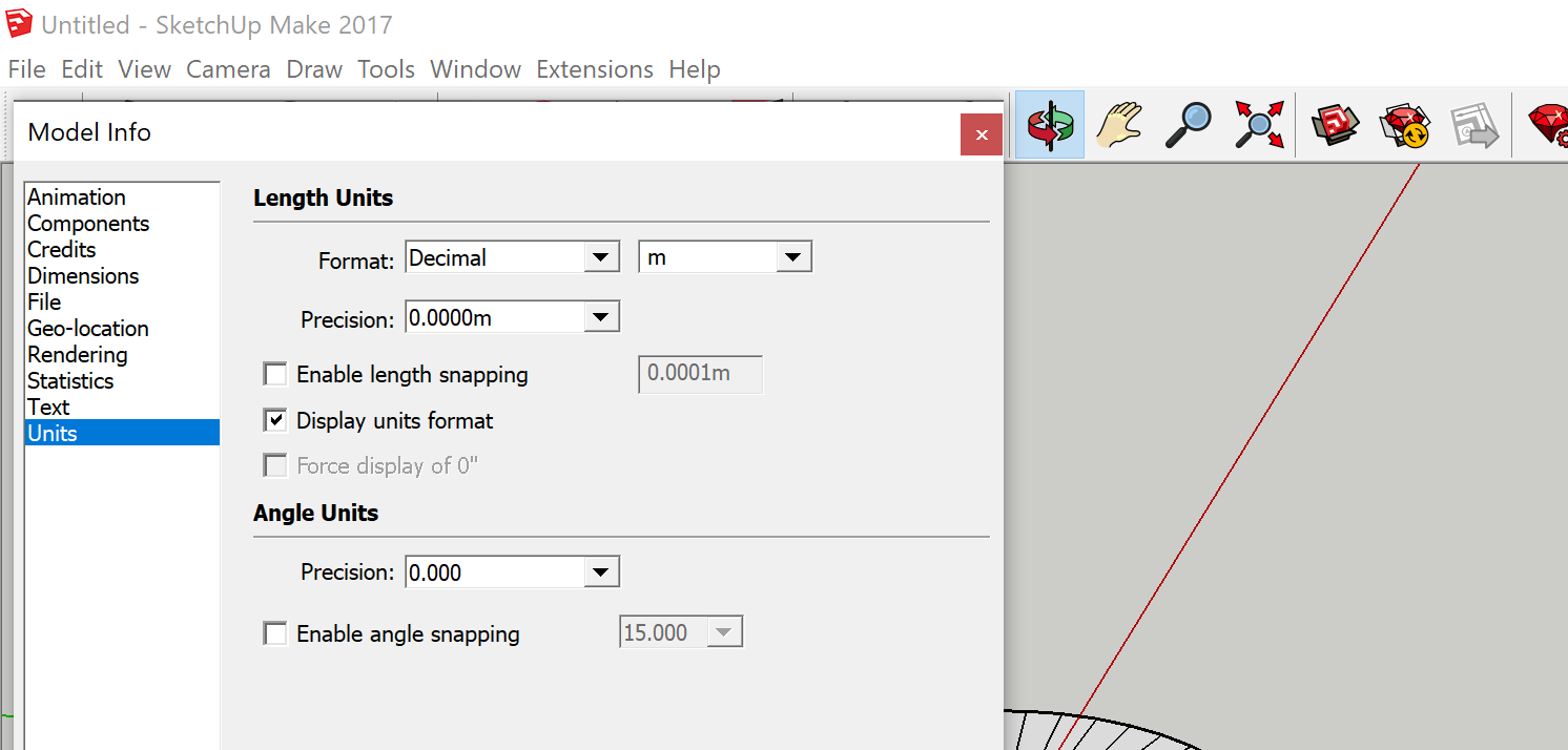
Sketchup Settings – Disable snapping

If you are like me then auto-snapping is often a huge pet peeve. To disable it, go to Model Info > Units and unclick Length snapping and Angle snapping.

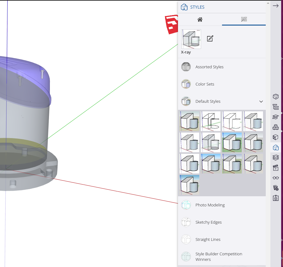
Sketchup Settings – Xray mode

It can be helpful to set the default view to xray mode so you can see inside the model when manipulating the components. To do this go to Styles > Default Styles > X-ray on the right hand side.

---

Generating component STL files

A common starting point for modeling is that you have a 3D model of the full robot. When this is the case, the first step in building a Mujoco model is to generate separate STL files for each of the components of the robot that you want to be able to move independently. For each of these component STL files, we want the point where it connects to the joint to be at the origin (0, 0, 0). We’ve found that this streamlines the process of building the model in the XML and makes it much easier to correctly specify the inertial properties.

If your 3D model is already broken up into each dynamic component (i.e. each arm section that moves independently) then you can skip to the section on centering at the origin.

Exporting components to separate STLs

Make sure you have the model unlocked. To do so, choose the Select tool and highlight the entire model. If the outline is red, it is locked. To unlock it, right click and choose Unlock.

Locked

Unlocked

Unlocking the UR5 model in SketchUp

To get each component piece: Select the entire arm, deselect your component with Ctrl + Shift + Click, and then delete the rest. Go to the folder icon in the top left and select Export > STL. When exporting your model, make sure to not save your model in ASCII format, choose Binary. Repeat this until you have exported every part as its own STL.

How to save an individual component from a complete robot model

Positioning your object at the origin

For each component, identify where it will connect to the previous component, i.e. where the joint will attach it to the rest of the robot. We want to set up the STL such that this point is at the origin. By doing this we simplify building the XML file later. For the base of the robot this would simply be the bottom of the link, centered.

The easiest way to move the object to the origin is to click a point on the object with the move tool, type [0, 0, 0], and hit enter. This will move the selected point to the origin.

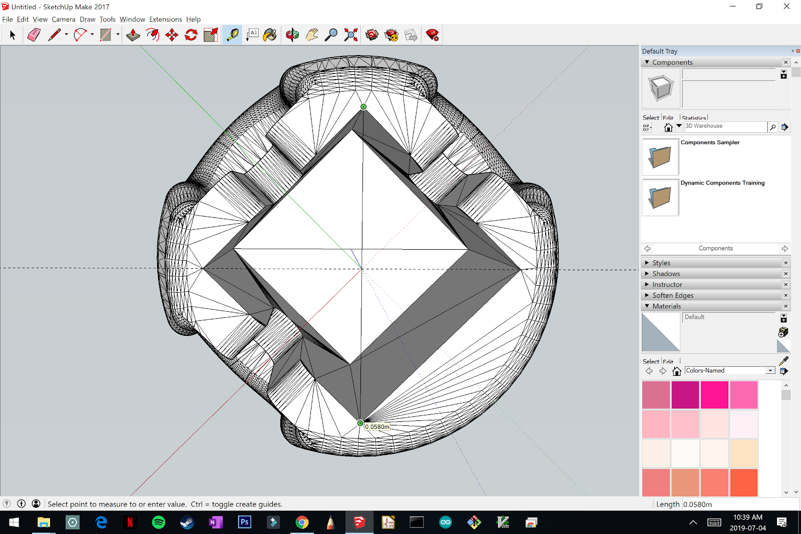
If your object is asymmetrical or you want to center on a point that is difficult to select with your mouse, you can use the measurement tool to set some guidelines. Setting two intersecting lines can help greatly in finding the center of an object (see dotted lines in figure).

Using dotted black guidelines to select an off-center point

Measure the offset distance for the next link

Once the component is appropriately placed at the origin, the next thing we need is the distance to the next attachment point from the origin.

The screenshots below show an example of drawing a verticle guideline to make selecting the next attachment point easy.

Making a verticle reference line that extends beyond the point of interest

Selecting the attachment point of the next component to measure the offset distance

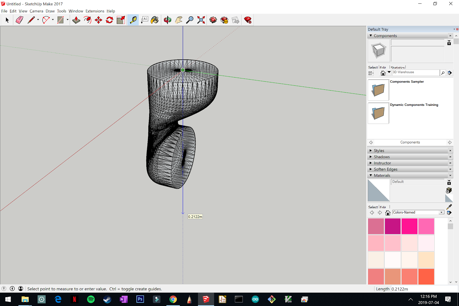
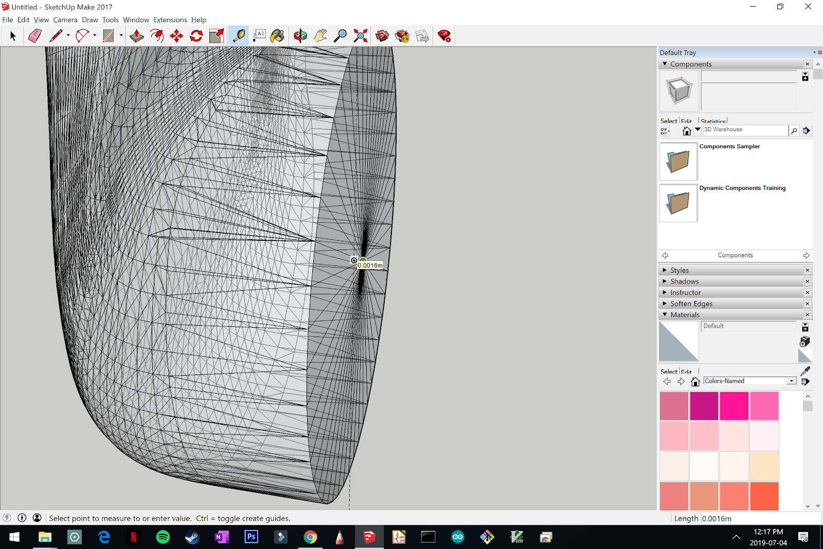
When the next attachment point is selected, the Measurements box will display its coordinates. We will need to know all of the offset distances for each component for building the XML file, so make sure you take note!

Some measuring tips

• Press and hold a directional button while measuring to lock an axis. The up arrow locks the z (blue) axis, the left arrow locks the y (green) axis, and the right arrow locks the x (red) axis.
• The measuring tape line changes color to match an axis colors when it is parallel to any axis.
• Notes on how to use the Tape Measure tool effectively

---

Building your model XML

The easiet way to put together your robot is to build your model up one joint and component at a time, running the simulation to make sure that it works as expected, and then adding the next piece. You will be tempted to assemble a bunch of the model all at once, but this is the siren’s song. You must be strong and resist!

For testing, we created the basic script below, which uses the ABR Control library. To check alignment you can press the space bar to pause the simulation, if you want to make the arm to move then you can change the script to send in some small value instead of zeros.

import mujoco_py as mjp
import glfw
import numpy as np

from abr_control.interfaces.mujoco import Mujoco
from abr_control.arms.mujoco_config import MujocoConfig

robot_config = MujocoConfig(xml_file='example.xml', folder='.')
interface = Mujoco(robot_config, dt=0.001)
interface.connect()

try:
    while True:
        if interface.viewer.exit:
            glfw.destroy_window(interface.viewer.window)
            break

        interface.send_forces(np.zeros(robot_config.N_JOINTS))

finally:
    interface.disconnect()

To run this script with your model, place it in the same directory as your XML file, with a folder called ‘meshes’ that has all of your STLs. If you call your XML file something other than ‘example.xml’ be sure to change that in the script above.

XML model parts

When you’re building your XML file, you’re going to want to have the Mujoco XML Reference constantly open. It’s super detailed and thorough. You can also check out this basic template file on my GitHub which shows the different parts of the file (you will need to fill this out with your own STLs and measurements).

Inside the standard definition tags, the main parts that we’ll be using are:

• <asset> – where you import your STLs using the <mesh> tag
• <worldbody> – where all of the objects in the simulation are defined using <body> tags, including lights, the floor, and of course your robot
• <acutator> – where you specify which joints defined in your robot can be actuated. The ordering of these joints is important, it should be the same as their order in the kinematic tree (i.e. start with joint0 up to the last joint.)

Body building

The meat of the file is of course in the sequence of <body> tags that define the robot model. Each section of the robot looks like this:

<body name="link_n" pos="0 0 0">
    <joint name="joint_n-1" axis="0 0 0" pos="0 0 0"/>
    <geom name="link_n" type="mesh" mesh="shoulder" pos="0 0 0" euler="0 0 0"/>
    <inertial pos="0 0 0" mass="0.01" diaginertia="0 0 0"/>

    <!-- nest the next joint here -->
</body>

Set body position and geoms
Set the offset from the previous body in the pos attribute on the <body> tag, instead of on the geoms. On the <joint> you can then set pos="0 0 0" which we’ve found to help simplify debugging later on.

In each body section you can have several <joint>s and <geom>s. Geoms defined on the same body will be fused together. If you have specific inertia properties for several geoms that are fused together, you will have to create a <body> for each to be able to instantiate their own <inertial> tag. Otherwise, it’s recommended to put them all in the same <body> to optimize simulation speed.

Orientation and inertia
You may need to rotate your STLs to align them properly with the rest of the robot as you build. You can do this either in the <body> or <geom> tags. If you are using an <inertial> tag for this body, we recommend you do this using the euler parameter inside the <geom> tag, instead of inside the <body> tag. If you specify rotation in the <body> tag, you also need to apply the same rotation to your <inertia> parameters, which complicates things.

If you don’t provide an <inertial> tag, the inertia properties will be inferred from the geom.

Contype and conaffinity
If you have geoms that you don’t want to collide with other parts in the model, you can set the contype and conaffinity parameters on the geom tags. This can be handy if you have a tightly-fit 3D model an run into issues with friction, we do this on the UR5 model in the ABR Control library.

End-effector tag for ABR Control
If you’re going to use the ABR Control library operational space controller, you’ll need to add a tag <body name="EE" pos="0 0 0"> at the point of the robot that you want to control. Usually the hand.

Once you’ve added on your robot body segment, save the XML and run the above python script to test out the set up. You will likely need to do some fine tuning by iteratively adjusting the parameters and viewing the model in Mujoco. We’ve found commenting out all of the joints except the joint of interest in the XML file makes assessment much easier.

Template XML file

<mujoco model="example">
    <!-- set some defaults for units and lighting -->
    <compiler angle="radian" meshdir="meshes"/>

    <!-- import our stl files -->
    <asset>
        <mesh file="base.STL" />
        <mesh file="link1.STL" />
        <mesh file="link2.STL" />
    </asset>

    <!-- define our robot model -->
    <worldbody>
        <!-- set up a light pointing down on the robot -->
        <light directional="true" pos="-0.5 0.5 3" dir="0 0 -1" />
        <!-- add a floor so we don't stare off into the abyss -->
        <geom name="floor" pos="0 0 0" size="1 1 1" type="plane" rgba="1 0.83 0.61 0.5"/>
        <!-- the ABR Control Mujoco interface expects a hand mocap -->
        <body name="hand" pos="0 0 0" mocap="true">
            <geom type="box" size=".01 .02 .03" rgba="0 .9 0 .5" contype="2"/>
        </body>

        <!-- start building our model -->
        <body name="base" pos="0 0 0">
            <geom name="link0" type="mesh" mesh="base" pos="0 0 0"/>
            <inertial pos="0 0 0" mass="0" diaginertia="0 0 0"/>

            <!-- nest each child piece inside the parent body tags -->
            <body name="link1" pos="0 0 1">
                <!-- this joint connects link1 to the base -->
                <joint name="joint0" axis="0 0 1" pos="0 0 0"/>

                <geom name="link1" type="mesh" mesh="link1" pos="0 0 0" euler="0 3.14 0"/>
                <inertial pos="0 0 0" mass="0.75" diaginertia="1 1 1"/>

                <body name="link2" pos="0 0 1">
                    <!-- this joint connects link2 to link1 -->
                    <joint name="joint1" axis="0 0 1" pos="0 0 0"/>

                    <geom name="link2" type="mesh" mesh="link2" pos="0 0 0" euler="0 3.14 0"/>
                    <inertial pos="0 0 0" mass="0.75" diaginertia="1 1 1"/>

                    <!-- the ABR Control Mujoco interface uses the EE body to -->
                    <!-- identify the end-effector point to control with OSC-->
                    <body name="EE" pos="0 0.2 0.2">
                        <inertial pos="0 0 0" mass="0" diaginertia="0 0 0" />
                    </body>
                </body>
            </body>
        </body>
    </worldbody>

    <!-- attach actuators to joints -->
    <actuator>
        <motor name="joint0_motor" joint="joint0"/>
        <motor name="joint1_motor" joint="joint1"/>
    </actuator>

</mujoco>

If you want to use the above template XML file with the example Mujoco simulation script withot having to create your own STLs, you can download the meshes folder from ABR Control’s Jaco 2 model to get going. The placement of things is wildly inaccurate but it’ll get you going. You can also checkout the abr_control/arms/jaco2/jaco2.xml and abr_control/arms/ur5/ur5.xml files for more examples.

Hopefully this is enough to get you started, if you run into questions you can post below or on the Mujoco forums. Happy modeling!

---

Troubleshooting

SketchUp – I’m importing my model but I can’t see it

It is likely that the units selected during the import were incorrect and the object is simply too small to see. When opening your STL, in the open file window select your file and click on the options button next to Import to change the units.

Mujoco – My arm isn’t moving, or moves slightly and stops

In this case you likely have collisions between links. You can either add a small gap between links (make sure to account for this shift in subsequent links and joints), or you can use the contype and conaffinity tags to set up the model such that collisions between the two components are not calculated.

For example, in our UR5 model, we set the touching geoms between links to have different contype and conaffinity values so that they don’t scrape against one another and prevent movement.

Mujoco – Parts of my model are spinning around wildly

This usually arises from being instantiated in contact with another part of the model. Sometimes it looks like there is clearly no contact between different model segments, but in fact there is because of how the contact dynamics are calculated.

Only convex shapes are supported. To see the shapes being used to calculate the contact dynamics, press F1 while the model is running. 

• 

  How the STL looks when it’s loaded, lots of space between the neck and jaw

• 

  The actual shapes that are used for calculating contact dynamics.

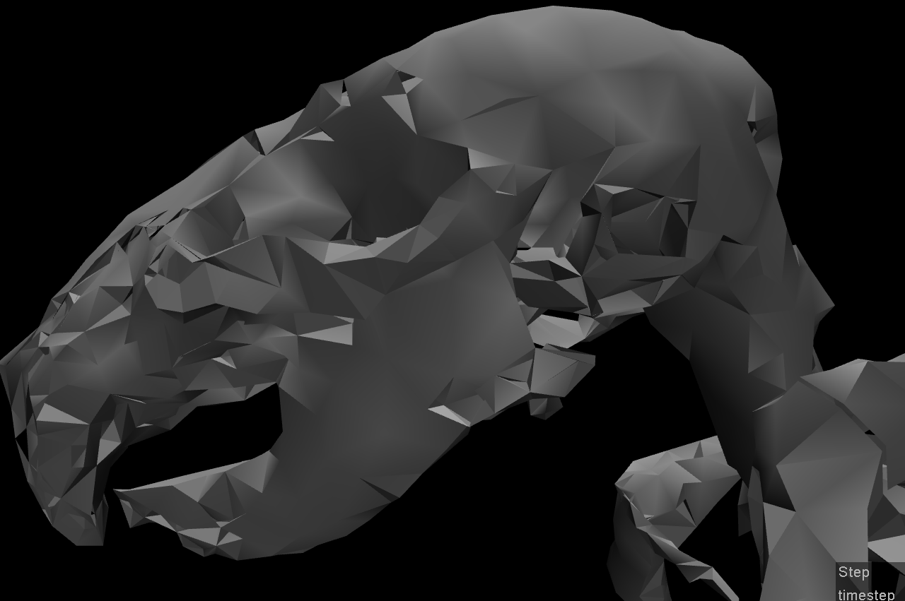
There is no space between the neck and jaw. To address this, you need break things up into multiple component STL files and then stitch them together in the XML. For example, in the above skeleton you would need to break it up into skull and spine STLs. NB: I will not be answering any questions about why a skeleton was used in this example.

Converting your Keras model into a spiking neural network

Let’s set the scene: You know Keras, you’ve heard about spiking neural networks (SNNs), and you want to see what all the fuss is about. For some reason. Maybe it’s to take advantage of some cool neuromorphic edge AI hardware, maybe you’re into computational modeling of the brain, maybe you’re masochistic and like a challenge, or you just think SNNs are cool. I won’t question your motives as long as you don’t start making jokes about SkyNet.

Welcome! In this post I’m going to walk through using Nengo DL to convert models built using Keras into SNNs. Nengo is neural modeling and runtime software built and maintained by Applied Brain Research. We started it and have been using it in the Computational Neuroscience Research Group for a long time now. Nengo DL lets you build neural networks using the Nengo API, and then run them using TensorFlow. You can run any kind of network you want in Nengo (ANNs, RNNs, CNNs, SNNs, etc), but here I’ll be focusing on SNNs.

There are a lot of little things to watch out for in this process. In this post I’ll work through the steps to convert and debug a simple network that classifies MNIST digits. The goal is to show you how you can start converting your own networks and some ways you can debug it if you encounter issues. Programming networks with temporal dynamics is a pretty unintuitive process and there’s lots of nuance to learn, but hopefully this will help you get started.

You can find an IPython notebook with all the code you need to run everything here up on my GitHub. The code I’ll be showing in this post is incomplete. I’m going to focus on the building, training, and conversion of the network and leave out parts like imports, loading in MNIST data, etc. To actually run this code you should get the IPython notebook, and make sure you have the latest Nengo, Nengo DL, and all the other dependencies installed.

Build your network in Keras and running it using NengoDL

The network is just going to be a convnet layer and then a fully connected layer. We build this in Keras all per uje … ushe … you-j … usual:

input = tf.keras.Input(shape=(28, 28, 1))
conv1 = tf.keras.layers.Conv2D(
    filters=32,
    kernel_size=3,
    activation=tf.nn.relu,
)(input)
flatten = tf.keras.layers.Flatten()(conv1)
dense1 = tf.keras.layers.Dense(units=10)(flatten)

model = tf.keras.Model(inputs=input, outputs=dense1)

Once the model is made we can generate a Nengo network from this by calling the NengoDL Converter. We pass the converted network into the Simulator, compile with the standard one-hot classification loss function, and start training.

converter = nengo_dl.Converter(
    model,
    swap_activations={tf.nn.relu: nengo.RectifiedLinear()},
)
net = converter.net
nengo_input = converter.inputs[input]
nengo_output = converter.outputs[dense1]

# run training
with nengo_dl.Simulator(net, seed=0) as sim:
    sim.compile(
        optimizer=tf.optimizers.RMSprop(0.001),
        loss={nengo_output: tf.losses.SparseCategoricalCrossentropy(from_logits=True)},
    )
    
    sim.fit(train_images, {nengo_output: train_labels}, epochs=10)

    # save the parameters to file
    sim.save_params("mnist_params")

In the Converter call you’ll see that there’s a swap_activations keyword. This is for us to map the TensorFlow activation functions to Nengo activation functions. In this case we’re just mapping ReLU to ReLU. After the training is done, we save the trained parameters to file.

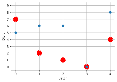
Next, we can load our trained parameters, call the sim.predict function and plot the results:

n_test = 5
with nengo_dl.Simulator(net, seed=0) as sim:
    sim.load_params(params_file)
    data = sim.predict({nengo_input: test_images[:n_test]})

# plot the answer in a big red x
plt.plot(test_labels[:n_test].squeeze(), 'rx', mew=15)
# data[nengo_output].shape = (images, timesteps, n_outputs)
# plot predicted digit from network output on the last time step
plt.plot(np.argmax(data[nengo_output][:, -1], axis=1), 'o', mew=2)

Red x’s are the answers, blue o’s are the network predictions.

NengoDL inherently accounts for time in its simulations and so the data all needs to be formatted as (n_batches, n_timesteps, n_inputs). In this case everything is using standard rate mode neurons with no internal states that change over time, so simulating the network over time will generate the same output at every time step. When we move to spiking neurons, however, effects of temporal dynamics will be visible.

Convert to spiking neurons

To convert our network to spiking neurons, all we have to do is change the neuron activation function that we map to in the converter when we’re generating the net:

converter = nengo_dl.Converter(
    model,
    swap_activations={tf.nn.relu: nengo.SpikingRectifiedLinear()},
)
net = converter.net
nengo_input = converter.inputs[input]
nengo_output = converter.outputs[dense1]

with nengo_dl.Simulator(net) as sim:
    sim.load_params("mnist_params")
    data = sim.predict({nengo_input: test_images[:n_test]})

So the process is that we create the model using Keras once. Then we can use a NengoDL Converter to create a Nengo network that can be simulated and trained. We save the parameters after training, and now we can use another Converter to create another instance of the network that uses SpikingRectifiedLinear neurons as the activation function. We can then load in the trained parameters that we got from simulating the standard RectifiedLinear rate mode activation function.

The reason that we don’t do the training with the SpikingRectifiedLinear activation function is because of its discontinuities, which cause errors when trying to calculate the derivative in backprop.

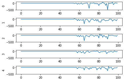
So! What kind of results do we get now that we’ve converted into spiking neurons?

Red x’s are the answers, blue o’s are the network predictions.

Not great! Why is this happening? Good question. It seems like what’s happening is the network is really convinced everything is 5. To investigate, we’re going to need to look at the neural activity.

Plotting the neural activity over time

To be able to see the activity of the neurons, we’re going to need 1) a reference to the ensemble of neurons we’re interested in monitoring, and 2) a Probe to track the activity of those neurons during simulation. This involves changing the network, so we’ll create another converted network and modify it before passing it into our Simulator.

converter = nengo_dl.Converter(
    model,
    swap_activations={tf.nn.relu: nengo.SpikingRectifiedLinear()},
)
net = converter.net

nengo_input = converter.inputs[input]
nengo_output = converter.outputs[dense1]
# get a reference for the neurons that we want to probe
nengo_conv1 = converter.layers[conv1]

# add probe to the network to track the activity of those neurons!
with converter.net as net:
    probe_conv1 = nengo.Probe(nengo_conv1, label='probe_conv1')

with nengo_dl.Simulator(net) as sim:
    sim.load_params("mnist_params")
    data = sim.predict({nengo_input: test_images[:n_test]})

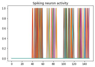
We can use Nengo’s handy rasterplot helper function to plot the activity of the first 3000 neurons:

from nengo.utils.matplotlib import rasterplot
# plot results neural activity from the first n_neurons on the
# first batch (each image is a batch), all time steps
rasterplot(np.arange(n_timesteps), data[probe_conv1][0, :, :n_neurons])

Raster plot of the spiking neural activity

If you have a keen eye and familiar with raster plots, you may notice that there are no spikes. Not a single one! So our network isn’t predicting a 5 for each input, it’s not predicting anything. We’re just getting 5 as output from a learned bias term. Bummer.

Let’s go back and see what kind of output our rate mode neurons are giving us, maybe that can help explain what’s going on. We can’t use a raster plot, because there are no spikes, but we can use a regular plot.

converter = nengo_dl.Converter(
    model,
    swap_activations={tf.nn.relu: nengo.RectifiedLinear()},
)
net = converter.net

nengo_input = converter.inputs[input]
nengo_output = converter.outputs[dense1]
nengo_conv1 = converter.layers[conv1]

with net:
    probe_conv1 = nengo.Probe(nengo_conv1)

with nengo_dl.Simulator(net) as sim:
    sim.load_params("mnist_params")
    data = sim.predict({nengo_input: test_images[:n_test]})

n_neurons = 5000
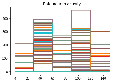
print('Max value: ', np.max(data[probe_conv1].flatten()))
# plot activity of first 5000 neurons, all inputs, all time steps
# we reshape the data so it's (n_batches * n_timesteps, n_neurons)
# for ease of plotting
plt.plot(data[probe_conv1][:, :, :n_neurons].reshape(-1, n_neurons))

Max value: 34.60704

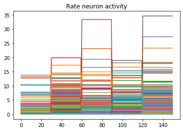
Looking at the rate mode activity of the neurons, we see that the max firing rate is 34.6Hz. That’s about 1 spike every 30 milliseconds. Through an unlucky coincidence we’ve set each image to be presented to the network for 30ms. What could be happening is that neurons are building up to the point of spiking, but the input is switched before they actually spike. To test this, let’s change the number of time steps each image is presented to 100ms, and rerun our spiking simulator.

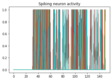
We’ll also switch over to plotting spiking activity the same way as the rate neurons for consistency (and because it’s easier to see if neurons are spiking or not when there’s really sparse activity). One thing you may note below is that I’m plotting activity * dt, instead of just activity like in the rate neuron case. Whenever there’s a spike in Nengo, it’s recorded as 1/dt so that it integrates to 1. Multiplying the probe output by dt means that we see a 1 when there’s one spike per time step, a 2 when there’s two spikes per time step, etc. It just makes it a bit easier to read.

print('Max value: ', np.max(data[probe_conv1].flatten() * dt))
print(data[probe_conv1][:,:,:n_neurons].shape)
plt.plot(data[probe_conv1][:, :, :n_neurons].reshape(-1, n_neurons) * dt)

• 

• 

Spiking network activity and output when images are presented for 100ms

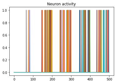
Looking at this plot, we can see a few things. First, whenever an image is presented, there’s a startup period where no spikes occur. Ideally our network will give us some output without having to present input for 50 time steps (the rate network gives us output after 1 time step!) We can address this by increasing the firing rates of the neurons in our network. We’ll come back to this.

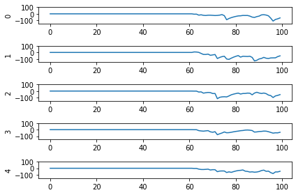
Second, even now that we’re getting spikes, the predictions for each image are very poor. Why is that happening? Let’s look at the network output over time when we feed in the first test image:

Output from the spiking network over 100ms (being shown a single image)

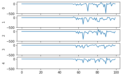
From this plot it looks like there’s not a clear prediction so much as a bunch of noise. One factor that can contribute to this is that the way things are set up right now, when a neuron spikes that information is only processed by the receiving side for 1 time step. Anthropomorphizing our network, you can think of the output layer as receiving input along the lines of “nothing … nothing … nothing … IT’S A 5! … maybe a 2? … maybe a 3? … IT’S A 5! ..” etc.

It would be useful for us to do a bit of averaging over time. Enter: synapses!

Using synapses to smooth the output of a spiking network

Synapses can come in many forms. The default form in Nengo is a low-pass filter. What this does for us is let the post-synaptic neuron (i.e. the neuron that we’re sending information to) do a bit of integration of the information that is being sent to it. So in the above example the output layer would be receiving input like “nothing … nothing … nothing … looking like a 5 … IT’S A 5! … it’s a 5! … it’s probably a 5 but maybe also a 2 or 3 … IT’S A 5! … ” etc.

Likely it will be more useful for understanding to see the actual network output over time with different low-pass filters applied rather than reading strained metaphors.

To make apply a low-pass filter synapse to all of the connections in our network is easy enough, we just add another modification to the network before passing it into the Simulator:

converter = nengo_dl.Converter(
    model,
    swap_activations={tf.nn.relu: nengo.SpikingRectifiedLinear()},
)
net = converter.net

nengo_input = converter.inputs[input]
nengo_output = converter.outputs[dense1]
nengo_conv1 = converter.layers[conv1]

with net:
    probe_conv1 = nengo.Probe(nengo_conv1)

# set a low-pass filter value on all synapses in the network
for conn in net.all_connections:
    conn.synapse = 0.001

with nengo_dl.Simulator(net) as sim:
    sim.load_params("mnist_params")
    data = sim.predict({nengo_input: test_images[:n_test]})

And here are the results we get for different low-pass filter time constants:

• 

• 

conn.synapse = None

• 

• 

conn.synapse = 0.001

• 

• 

conn.synapse = 0.005

• 

• 

conn.synapse = 0.01

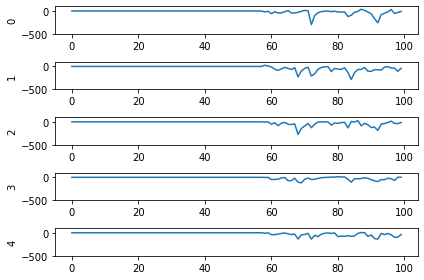
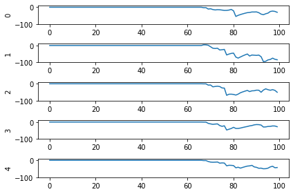
As the time constant on the low-pass filter increases, we can see the output of the network starts smoothing out. It’s important to recognize that there are a few things going on though when we filter values on all of the synapses of the network. The first is that we’re no longer sending sharp spikes between layers, we’re now passing along filtered spikes. The larger the time constant on the filter, the more spread out and smoother the signal will be.

As a result of this: If sending a spike from neuron A to neuron B used to cause neuron B to spike immediately when there was no synaptic filter, that may no longer be the case. It may now take several spikes from neuron A, all close together in time, for neuron B to now spike.

Another thing we want to consider is that we’ve applied a synaptic filter at every layer, so the dynamics of the entire network have changed. Very often you’ll want to be more surgical with the synapses you create, leaving some connections with no synapse and some with large filters to get the best performance out of your network. Currently the way to do this is to print out net.all_connections, find the connections of interest, and then index in specific values. When we print out net.all_connections for this network, we get:

[<Connection at 0x7fd8ac65e4a8 from <Node "conv2d.0.bias"> to <Node (unlabeled) at 0x7fd8ac65ee48>>,
<Connection at 0x7fd969a06b70 from <Node (unlabeled) at 0x7fd8ac65ee48> to <Neurons of <Ensemble "conv2d.0">>>,
<Connection at 0x7fd969a06390 from <Node "input_1"> to <Neurons of <Ensemble "conv2d.0">>>,
<Connection at 0x7fd8afc41470 from <Node "dense.0.bias"> to <Node "dense.0">>,
<Connection at 0x7fd8afc41588 from <Neurons of <Ensemble "conv2d.0">> to <Node "dense.0">>]

The connections of interest for us are from input_1 to conv2d.0, and from conv2d.0 to dense.0. These are the connections the input signals for the network are flowing through, the rest of the connections are just to send in trained bias values to each layer. We can set the synapse value for these connections specifically with the following:

synapses = [None, None, 0.001, None, 0.001]
for conn, synapse in zip(net.all_connections, synapses):
    conn.synapse = synapse

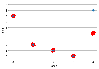
In this case, with just some playing around with different values I wasn’t able to find any synapse values that got better performance than 4/5. But in general being able to set specific synapse values in a spiking neural network is important and you should be aware of how to do it to get the best performance out of your network.

So setting the synapses is able to improve the performance of the network. We’re still taking 100ms to generate output though, and only getting 4/5 of the test set correct. Let’s go back now to the first issue we identified and look at increasing the firing rates of the neurons.

Increasing the firing rates of neurons in the network

There are a few ways to go about this. The first is a somewhat cheeky method that works best for rectified linear (ReLU) neurons, and the second is a more general method that adjusts how training is performed.

Scaling ReLU firing rates

Because we’re using rectified linear neurons in this model, one trick that we can use to increase the firing rates without affecting the functionality of the network is by using a scaling term to multiply the input and divide the output of each neuron. This scaling can work because the rectified linear neuron model is linear in its activation function.

The result of this scaling is more frequent spiking at a lower amplitude. We can implement this using the Nengo DL Converter with the scale_firing_rates keyword:

converter = nengo_dl.Converter(
    model,
    swap_activations={tf.nn.relu: nengo.SpikingRectifiedLinear()},
    scale_firing_rates=gain_scale,
)

Let’s look at the network output and neural activity plots for gain_scale values of [5, 20, 50].

• 

• 

gain_scale = 5

• 

• 

gain_scale = 20

• 

• 

gain_scale = 50

One thing that’s apparent is as the firing rates go up, the performance of the network gets better. You may notice that for the first image (first 30 time steps) in the spiking activity plots there’s no response. Don’t read too much into that; I’m plotting a random subset of neurons and it just happens that none of them respond to the first image. If I was to plot the activity of all of the neurons we’d see spikes everywhere.

You may also notice that when gain_scale = 50 we’re even getting some neurons that are spiking 2 times per time step. That will happen when the input to the neuron causes the internal state to jump up to twice the threshold for spiking for that neuron. This is not unexpected behaviour.

Using this scale_firing_rates keyword in the Converter is one way to get the performance of our coverted spiking networks to match the performance of rate neuron networks. However, it mainly a trick useful for us for ReLUs (and any other linear activation functions). It would behoove us to figure out another method that will work as well for nonlinear activation functions as well.

Adding a firing rate term to the cost function during training

Let’s go back to the training the network step. Another way to bring the firing rates up is by adding a term to the cost function that will penalize any firing rates outside of some desired range. There are a ton of ways to go about this with different kinds of cost functions. I’m just going to present one cost function term that works for this situation and note that you can build this cost function a whole bunch of different ways. Here’s one:

def put_in_range(x, y, weight=100.0, min=200, max=300):
    index_greater = (y > max)  # find neurons firing faster
    index_lesser = (y < min)  # find neurons firing slower
    error = tf.reduce_sum(y[index_greater] - max) + tf.reduce_sum(min - y[index_lesser])
    return weight * error

The weight parameter lets us set the relative importance of the firing rates cost function term relative to the classification accuracy cost function term. To use this term we need to make a couple of adjustments to our code for training the network:

converter = nengo_dl.Converter(
    model,
    swap_activations={tf.nn.relu: nengo.RectifiedLinear()},
)
net = converter.net

nengo_input = converter.inputs[input]
nengo_output = converter.outputs[dense1]

nengo_conv1 = converter.layers[conv1]
with converter.net as net:
    probe_conv1 = nengo.Probe(nengo_conv1, label='probe_conv1')

# run training
with nengo_dl.Simulator(net) as sim:
    sim.compile(
        optimizer=tf.optimizers.RMSprop(0.001),
        loss={
            nengo_output: tf.losses.SparseCategoricalCrossentropy(from_logits=True),
            probe_conv1: put_in_range,
        }
    )
    sim.fit(
        train_images,
        {nengo_output: train_labels, 
         probe_conv1: np.zeros(train_labels.shape)},
        epochs=10)

Mainly what’s been added in this code is our new loss function put_in_range and in the sim.compile call we added probe_conv1: put_in_range to the loss dictionary. This tells Nengo DL to use the put_in_range cost function on the output from probe_conv1, which will be the firing rates of the convolutional layer of neurons in the network.

We also had to add in probe_conv1: np.zeros(train_labels.shape) to the input dictionary in the sim.fit function call. The array specified here is used as the x input to the put_in_range cost function, but since we defined the put_in_range function to be fully determined based only on y (which is the output from probe_conv1) it doesn’t matter what values we pass in there. So I pass in an array of zeros.

Now when we run the training and prediction in rate mode, the output we get looks like

• 

• 

Rate network output with put_in_range term added to cost function

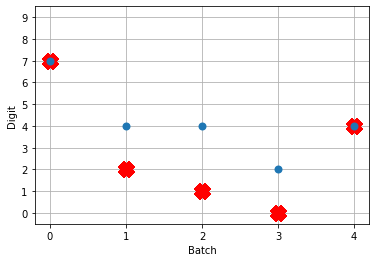
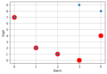
And we can see that we’re still getting the same performance, but now the firing rates of the neurons are much higher. Let’s see what happens when we convert to spiking neurons now!

• 

• 

Spiking network output with put_in_range term added to cost function

Hey, that’s looking much better! This of course is only looking at 5 test images and you’ll want to go through and calculate proper performance statistics using a full test set, but it’s a good start.

Conclusions

This post has looked at how to take a model that you built in Keras and convert it over to a spiking neural network using Nengo DL’s Converter function. This was a simple model, but hopefully it gets across that the conversion to spikes can be an iterative process, and you now have a better sense of some of the steps that you can take to investigate and debug spiking neural network behaviour! In general when tuning your network you’ll use a mix of the different methods we’ve gone through here, depending on the exact situation.

Again a reminder that all of the code for this can be found up on my GitHub.

Also! It’s very much worth checking out the Nengo DL documentation and other examples that they have there. There’s a great introduction for users coming from TensorFlow over to Nengo, and other examples showing how you can integrate non-spiking networks with spiking networks, as well as other ways to optimizing your spiking neural networks. If you start playing around with Nengo and have more questions, please feel free to ask in comments below or even better go to the Nengo forums!

Force control of task-space orientation

So you want to use force control to control the orientation of your end-effector, eh? What a noble endeavour. I, too, wished to control the orientation of the end-effector. While the journey was long and arduous, the resulting code is short and quick to implement. All of the code for reproducing the results shown here is up on my GitHub and in the ABR Control repo. 

Introduction

There are numerous resources that introduce the topic of orientation control, so I’m not going to do a full rehash here. I will link to resources that I found helpful, but a quick google search will pull up many useful references on the basics. 

When describing the orientation of the end-effector there are three different primary methods used: Euler angles, rotation matrices, and quaternions. The Euler angles , and denote roll, pitch, and yaw, respectively. Rotation matrices specify 3 orthogonal unit vectors, and I describe in detail how to calculate them in this post on forward transforms. And quaternions are 4-dimensional vectors used to describe 3 dimensional orientation, which provide stability and require less memory and compute but are more complicated to understand.

Most modern robotics control is done using quaternions because they do not have singularities, and it is straight forward to convert them to other representations. Fun fact: Quaternion trajectories also interpolate nicely, where Euler angles and rotation matrices do not, so they are used in computer graphics to generate a trajectory for an object to follow in orientation space.

While you won’t need a full understanding of quaternions to use the orientation control code, it definitely helps if anything goes wrong. If you are looking to learn about or brush up on quaternions, or even if you’re not but you haven’t seen this resource, you should definitely check out these interactive videos by Grant Sanderson and Ben Eater. They have done an incredible job developing modules to give people an intuition into how quaternions work, and I can’t recommend their work enough. There’s also a non-interactive video version that covers the same material.

In control literature, angular velocity and acceleration are denoted and . It’s important to remember that is denoting a velocity, and not a position, as we work through things or it could take you a lot longer to understand than it otherwise might…

How to generate task-space angular forces

So, if you recall a post long ago on Jacobians, our task-space Jacobian has 6 rows:

In position control, where we’re only concerned about the position of the hand, the angular velocity dimensions are stripped out of the Jacobian so that it’s a 3 x n_joints matrix rather than a 6 x n_joints matrix. So the orientation of the end-effector is not controlled at all. When we did this, we didn’t need to worry or know anything about the form of the angular velocities.

Now that we’re interested in orientation control, however, we will need to learn up (and thank you to Yitao Ding for clarifying this point in comments on the original version of this post). The Jacobian for the orientation describes the rotational velocities around each axis with respect to joint velocities. The rotational velocity of each axis “happens” at the same time. It’s important to note that this is not the same thing as Euler angles, which are applied sequentially.

To generate our task-space angular forces we will have to generate an orientation angle error signal of the appropriate form. To do that, first we’re going to have to get and be able to manipulate the orientation representation of the end-effector and our target.

Transforming orientation between representations

We can get the current end-effector orientation in rotation matrix form quickly, using the transformation matrices for the robot. To get the target end-effector orientation in the examples below we’ll use the VREP remote API, which returns Euler angles.

It’s important to note that Euler angles can come in 12 different formats. You have to know what kind of Euler angles you’re dealing with (e.g. rotate around X then Y then Z, or rotate around X then Y then X, etc) for all of this to work properly. It should be well documented somewhere, for example the VREP API page tells us that it will return angles corresponding to x, y, and then z rotations.

The axes of rotation can be static (extrinsic rotations) or rotating (intrinsic rotations). NOTE: The VREP page says that they rotate around an absolute frame of reference, which I take to mean static, but I believe that’s a typo on their page. If you calculate the orientation of the end-effector of the UR5 using transform matrices, and then convert it to Euler angles with axes='rxyz' you get a match with the displayed Euler angles, but not with axes='sxyz'.

Now we’re going to have to be able to transform between Euler angles, rotation matrices, and quaternions. There are well established methods for doing this, and a bunch of people have coded things up to do it efficiently. Here I use the very handy transformations module from Christoph Gohlke at the University of California. Importantly, when converting to quaternions, don’t forget to normalize the quaternions to unit length.

from abr_control.arms import ur5 as arm
from abr_control.interfaces import VREP
from abr_control.utils import transformations

robot_config = arm.Config()
interface = VREP(robot_config)
interface.connect()

feedback = interface.get_feedback()
# get the end-effector orientation matrix
R_e = robot_config.R('EE', q=feedback['q'])
# calculate the end-effector unit quaternion
q_e = transformations.unit_vector(
    transformations.quaternion_from_matrix(R_e))

# get the target information from VREP
target = np.hstack([
    interface.get_xyz('target'),
    interface.get_orientation('target')])
# calculate the target orientation rotation matrix
R_d = transformations.euler_matrix(
    target[3], target[4], target[5], axes='rxyz')[:3, :3]
# calculate the target orientation unit quaternion
q_d = transformations.unit_vector(
    transformations.quaternion_from_euler(
        target[3], target[4], target[5],
        axes='rxyz'))  # converting angles from 'rotating xyz'

Generating the orientation error

I implemented 4 different methods for calculating the orientation error, from (Caccavale et al, 1998), (Yuan, 1988) and (Nakinishi et al, 2008), and then one based off some code I found on Stack Overflow. I’ll describe each below, and then we’ll look at the results of applying them in VREP.

Method 1 – Based on code from StackOverflow

Given two orientation quaternion and , we want to calculate the rotation quaternion that takes us from  to :

To isolate , we right multiply by the inverse of . All orientation quaternions are of unit length, and for unit quaternions the inverse is the same as the conjugate. To calculate the conjugate of a quaternion, denoted here, we negate either the scalar or vector part of the quaternion, but not both.

Great! Now we know how to calculate the rotation needed to get from the current orientation to the target orientation. Next, we have to get from a set of target Euler angle forces. In A new method for performing digital control system attitude computations using quaternions (Ickes, 1968), he mentions mention that

For control purposes, the last three elements of the quaternion define the roll, pitch, and yaw rotational errors…

So you can just take the vector part of the quaternion and use that as your desired Euler angle forces.

# calculate the rotation between current and target orientations
q_r = transformations.quaternion_multiply(
    q_target, transformations.quaternion_conjugate(q_e))

# convert rotation quaternion to Euler angle forces
u_task[3:] = ko * q_r[1:] * np.sign(q_r[0])

NOTE: You will run into issues when the angle is crossed where the arm ‘goes the long way around’. To account for this, use q_r[1:] * np.sign(q_r[0]). This will make sure that you always rotate along a trajectory < 180 degrees towards the target angle. The reason that this crops up is because there are multiple different quaternions that can represent the same orientation.

The following figure shows the arm being directed from and to the same orientations, where the one on the left takes the long way around, and the one on the right multiplies by the sign of the scalar component of the quaternion as specified above.

• 

• 

---

Method 2 – Quaternion feedback from Resolved-acceleration control of robot manipulators: A critical review with experiments (Caccavale et al, 1998)

In section IV, equation (34) of this paper they specify the orientation error to be calculated as

where is the rotation matrix for the end-effector, and is the vector part of the unit quaternion that can be extracted from the rotation matrix

.

To implement this is pretty straight forward using the transforms.py module to handle the representation conversions:

# From (Caccavale et al, 1997)
# Section IV - Quaternion feedback
R_ed = np.dot(R_e.T, R_d)  # eq 24
q_ed = transformations.quaternion_from_matrix(R_ed)
q_ed = transformations.unit_vector(q_ed)
u_task[3:] = -np.dot(R_e, q_ed[1:])  # eq 34

---

Method 3 – Angle/axis feedback from Resolved-acceleration control of robot manipulators: A critical review with experiments (Caccavale et al, 1998)

In section V of the paper, they present an angle / axis feedback algorithm, which overcomes the singularity issues that classic Euler angle methods suffer from. The algorithm defines the orientation error in equation (45) to be calculated

,

where and are the scalar and vector part of the quaternion representation of 

Where is the rotation matrix representing the desired orientation and is the rotation matrix representing the end-effector orientation. The code implementation for this looks like:

# From (Caccavale et al, 1997)
# Section V - Angle/axis feedback
R_de = np.dot(R_d, R_e.T)  # eq 44
q_ed = transformations.quaternion_from_matrix(R_de)
q_ed = transformations.unit_vector(q_ed)
u_task[3:] = -2 * q_ed[0] * q_ed[1:]  # eq 45

From playing around with this briefly, it seems like this method also works. The authors note in the discussion that it may “suffer in the case of large orientation errors”, but I wasn’t able to elicit poor behaviour when playing around with it in VREP. The other downside they mention is that the computational burden is heavier with this method than with quaternion feedback.

---

Method 4 – From Closed-loop manipulater control using quaternion feedback (Yuan, 1988) and Operational space control: A theoretical and empirical comparison (Nakanishi et al, 2008)

This was the one method that I wasn’t able to get implemented / working properly. Originally presented in (Yuan, 1988), and then modified for representing the angular velocity in world and not local coordinates in (Nakanishi et al, 2008), the equation for generating error (Nakanishi eq 72):

where and are the scalar and vector components of the quaternions representing the end-effector and target orientations, respectively, and is defined in (Nakanishi eq 73):

My code for this implementation looks like:

S = np.array([
    [0.0, -q_d[2], q_d[1]],
    [q_d[2], 0.0, -q_d[0]],
    [-q_d[1], q_d[0], 0.0]])

u_task[3:] = -(q_d[0] * q_e[1:] - q_e[0] * q_d[1:] +
               np.dot(S, q_e[1:]))

If you understand why this isn’t working, if you can provide a working code example in the comments I would be very grateful.

---

Generating the full orientation control signal

The above steps generate the task-space control signal, and from here I’m just using standard operational space control methods to take u_task and transform it into joint torques to send out to the arm. With possibly the caveat that I’m accounting for velocity in joint-space, not task space. Generating the full control signal looks like:

 
# which dim to control of [x, y, z, alpha, beta, gamma]
ctrlr_dof = np.array([False, False, False, True, True, True])

feedback = interface.get_feedback()
# get the end-effector orientation matrix
R_e = robot_config.R('EE', q=feedback['q'])
# calculate the end-effector unit quaternion
q_e = transformations.unit_vector(
    transformations.quaternion_from_matrix(R_e))

# get the target information from VREP
target = np.hstack([
    interface.get_xyz('target'),
    interface.get_orientation('target')])
# calculate the target orientation rotation matrix
R_d = transformations.euler_matrix(
    target[3], target[4], target[5], axes='rxyz')[:3, :3]
# calculate the target orientation unit quaternion
q_d = transformations.unit_vector(
    transformations.quaternion_from_euler(
        target[3], target[4], target[5],
        axes='rxyz'))  # converting angles from 'rotating xyz'

# calculate the Jacobian for the end effectora
# and isolate relevate dimensions
J = robot_config.J('EE', q=feedback['q'])[ctrlr_dof]

# calculate the inertia matrix in task space
M = robot_config.M(q=feedback['q'])

# calculate the inertia matrix in task space
M_inv = np.linalg.inv(M)
Mx_inv = np.dot(J, np.dot(M_inv, J.T))
if np.linalg.det(Mx_inv) != 0:
    # do the linalg inverse if matrix is non-singular
    # because it's faster and more accurate
    Mx = np.linalg.inv(Mx_inv)
else:
    # using the rcond to set singular values < thresh to 0
    # singular values < (rcond * max(singular_values)) set to 0
    Mx = np.linalg.pinv(Mx_inv, rcond=.005)

u_task = np.zeros(6)  # [x, y, z, alpha, beta, gamma]

# generate orientation error
# CODE FROM ONE OF ABOVE METHODS HERE

# remove uncontrolled dimensions from u_task
u_task = u_task[ctrlr_dof]

# transform from operational space to torques and
# add in velocity and gravity compensation in joint space
u = (np.dot(J.T, np.dot(Mx, u_task)) -
     kv * np.dot(M, feedback['dq']) -
     robot_config.g(q=feedback['q']))

# apply the control signal, step the sim forward
interface.send_forces(u)

The control script in full context is available up on my GitHub along with the corresponding VREP scene. If you download and run both (and have the ABR Control repo installed), then you can generate fun videos like the following:

• 

  Method 1 – Stack overflow code

• 

  Method 2 – Caccavale quaternion

• 

  Method 3 – Caccavale angle/axis

• 

  Method 4 – Yuan / Nakanishi

Here, the green ball is the target, and the end-effector is being controlled to match the orientation of the ball. The blue box is just a visualization aid for displaying the orientation of the end-effector. And that hand is on there just from another project I was working on then forgot to remove but already made the videos so here we are. It’s set to not affect the dynamics so don’t worry. The target changes orientation once a second. The orientation gain for these trials is ko=200 and kv=np.sqrt(600).

The first three methods all perform relatively similarly to each other, although method 3 seems to be a bit faster to converge to the target orientation after the first movement. But it’s pretty clear something is terribly wrong with the implementation of the Yuan algorithm in method 4; brownie points for whoever figures out what!

Controlling position and orientation

So you want to use force control to control both position and orientation, eh? You are truly reaching for the stars, and I applaud you. For the most part, this is pretty straight-forward. But there are a couple of gotchyas so I’ll explicitly go through the process here.

How many degrees-of-freedom (DOF) can be controlled?

If you recall from my article on Jacobians, there was a section on analysing the Jacobian. It comes down to two main points: 1) The Jacobian specifies which task-space DOF can be controlled. If there is a row of zeros, for example, the corresponding task-space DOF (i.e. cannot be controlled. 2) The rank of the Jacobian determines how many DOF can be controlled at the same time.

For example, in a two joint planar arm, the variables can be controlled, but cannot be controlled because their corresponding rows are all zeros. So 3 variables can potentially be controlled, but because the Jacobian is rank 2 only two variables can be controlled at a time. If you try to control more than 2 DOF at a time things are going to go poorly. Here are some animations of trying to control 3 DOF vs 2 DOF in a 2 joint arm:

• 

  controlling 3 DOF

• 

  controlling 2 DOF

How to specify which DOF are being controlled?

Okay, so we don’t want to try to control too many DOF at once. Got it. Let’s say we know that our arm has 3 DOF, how do we choose which DOF to control? Simple: You remove the rows from you Jacobian and your control signal that correspond to task-space DOF you don’t want to control.

To implement this in code in a flexible way, I’ve chosen to specify an array with 6 boolean elements, set to True if you want to control the corresponding task space parameter and False if you don’t. For example, if you to control just the parameters, you would set ctrl_dof = [True, True, True, False, False, False].

We then strip the Jacobian and task space control signal down to the relevant rows with J = robot_config.('EE', q)[ctrlr_dof] and u_task = (current - target)[ctrlr_dof]. This means that both current and target must be 6-dimensional vectors specifying the current and target values, respectively, regardless of how many dimensions we’re actually controlling.

Generating a position + orientation control signal

The UR5 has 6 degrees of freedom, so we’re able to fully control the task space position and orientation. To do this, in the above script just ctrl_dof = np.array([True, True, True, True, True, True]), and there you go! In the following animations the gain values used were kp=300, ko=300, and kv=np.sqrt(kp+ko)*1.5. The full script can be found up on my GitHub.

• 

  Method 1 – Stack overflow code

• 

  Method 2 – Caccavale quaternion

• 

  Method 3 – Caccavale angle/axis

• 

  Method 4 – Yuan / Nakanishi

NOTE: Setting the gains properly for this task is pretty critical, and I did it just by trial and error until I got something that was decent for each. For a real comparison, better parameter tuning would have to be undertaken more rigorously. 

NOTE: When implementing this minimal code example script I ran into a problem that was caused by the task-space inertia matrix calculation. It turns out that using np.linalg.pinv gives very different results than np.linalg.inv, and I did not realise this. I’m going to have to explore this more fully later, but basically heads up that you want to be using np.linalg.inv as much as possible. So you’ll notice in the above code I check the dimensionality of Mx_inv and first try to use np.linalg.inv before resorting to np.linalg.pinv.

NOTE: If you start playing around with controlling only one or two of the orientation angles, something to keep in mind: Because we’re using rotating axes, if you set up False, False, True then it’s not going to look like of the end-effector is lining up with the of the target. This is because and weren’t set first. If you generate a plot of the target orientations vs the end-effector orientations, however, you’ll see that you are in face reaching the target orientation for .

In summary

So that’s that! Lots of caveats, notes, and more work to be done, but hopefully this will be a useful resource for any others embarking on the same journey. You can download the code, try it out, and play around with the gains and targets. Let me know below if you have any questions or enjoyed the post, or want to share any other resources on force control of task-space orientation.

And once again thanks to Yitao Ding for his helpful comments and corrections on the original version of this article.

Natural policy gradient in TensorFlow

In working towards reproducing some results from deep learning control papers, one of the learning algorithms that came up was natural policy gradient. The basic idea of natural policy gradient is to use the curvature information of the of the policy’s distribution over actions in the weight update. There are good resources that go into details about the natural policy gradient method (such as here and here), so I’m not going to go into details in this post. Rather, possibly just because I’m new to TensorFlow, I found implementing this method less than straightforward due to a number of unexpected gotchyas. So I’m going to quickly review the algorithm and then mostly focus on the implementation issues that I ran into.

If you’re not familiar with policy gradient or various approaches to the cart-pole problem I also suggest that you check out this blog post from KV Frans, which provides the basis for the code I use here. All of the code that I use in this post is available up on my GitHub, and it’s worth noting this code is for TensorFlow 1.7.0.

Natural policy gradient review

Let’s informally define our notation

• and are the system state and chosen action at time
• are the network parameters that we’re learning
• is the control policy network parameterized
• is the advantage function, which returns the estimated total reward for taking action in state relative to default behaviour (i.e. was this action better or worse than what we normally do)

The regular policy gradient is calculated as:

where denotes calculating the partial derivative with respect to , the hat above denotes that we’re using an estimation of the advantage function, and returns a scalar value which is the probability of the chosen action in state .

For the natural policy gradient, we’re going to calculate the Fisher information matrix, , which estimates the curvature of the control policy:

The goal of including curvature information is to be able move along the steepest ascent direction, which we estimate with . Including this then the weight update becomes

where is a learning rate parameter. In his paper Towards Generalization and Simplicity in Continuous Control, Aravind Rajeswaran notes that empirically it’s difficult to choose an appropriate value or set an appropriate schedule. To address this, they normalize the update under the Fisher metric:

Using the above for the learning rate can be thought of as choosing a step size that is normalized with respect to the change in the control policy. This is beneficial because it means that we don’t do any parameter updates that will drastically change the output of the policy network.

Here’s what the pseudocode for the algorithm looks like

• Initialize policy parameters
• for k = 1 to K do:
  • collect N trajectories by rolling out the stochastic policy
  • compute for each pair along the trajectories sampled
  • compute advantages based on the sampled trajectories and the estimated value function
  • compute the policy gradient as specified above
  • compute the Fisher matrix and perform the weight update as specified above
  • update the value network to get

OK great! On to implementation.

Implementation in TensorFlow 1.7.0

Calculating the gradient at every time step

In TensorFlow, the tf.gradient(ys, xs) function, which calculates the partial derivative of  ys with respect to xs:

will automatically sum over over all elements in ys. There is no function for getting the gradient of each individual entry (i.e. the Jacobian) in ys, which is less than great. People have complained, but until some update happens we can address this with basic list comprehension to iterate through each entry in the history and calculate the gradient at that point in time. If you have a faster means that you’ve tested please comment below!

The code for this looks like

        g_log_prob = tf.stack(
            [tf.gradients(action_log_prob_flat[i], my_variables)[0]
                for i in range(action_log_prob_flat.get_shape()[0])])

Where the result is called g_log_prob_flat because it’s the gradient of the log probability of the chosen action at each time step.

Inverse of a positive definite matrix with rounding errors

One of the problems I ran into was in calculating the normalized learning rate was that the square root calculation was dying because negative values were being set in. This was very confusing because is a positive definite matrix, which means that is also positive definite, which means that for any .

So it was clear that it was a calculation error somewhere, but I couldn’t find the source of the error for a while, until I started doing the inverse calculation myself using SVD to explicitly look at the eigenvalues and make sure they were all > 0. Turns out that there were some very, very small eigenvalues with a negative sign, like -1e-7 kind of range. My guess (and hope) is that these are just rounding errors, but they’re enough to mess up the calculations of the normalized learning rate. So, to handle this I explicitly set those values to zero, and that took care of that.

        S, U, V = tf.svd(F)
        atol = tf.reduce_max(S) * 1e-6
        S_inv = tf.divide(1.0, S)
        S_inv = tf.where(S < atol, tf.zeros_like(S), S_inv)
        S_inv = tf.diag(S_inv)
        F_inv = tf.matmul(S_inv, tf.transpose(U))
        F_inv = tf.matmul(V, F_inv)

Manually adding an update to the learning parameters

Once the parameter update is explicitly calculated, we then need to update them. To implement an explicit parameter update in TensorFlow we do

        # update trainable parameters
        my_variables[0] = tf.assign_add(my_variables[0], update)

So to update the parameters then we call sess.run(my_variables, feed_dict={...}). It’s worth noting here too that any time you run the session with my_variables the parameter update will be calculated and applied, so you can’t run the session with my_variables to only fetch the current values.

Results on the CartPole problem

Now running the original policy gradient algorithm against the natural policy gradient algorithm (with everything else the same) we can examine the results of using the Fisher information matrix in the update provides some strong benefits. The plot below shows the maximum reward received in a batch of 200 time steps, where the system receives a reward of 1 for every time step that the pole stays upright, and 200 is the maximum reward achievable.

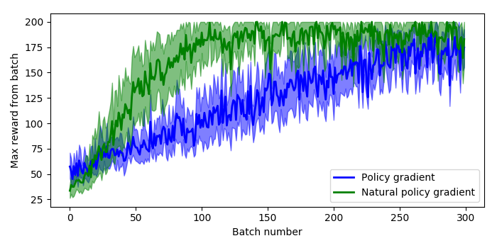
To generate this plot I ran 10 sessions of 300 batches, where each batch runs as many episodes as it takes to get 200 time steps of data. The solid lines are the mean value at each epoch across all sessions, and the shaded areas are the 95% confidence intervals. So we can see that the natural policy gradient starts to hit a reward of 200 inside 100 batches, and that the mean stays higher than normal policy gradient even after 300 batches.

It’s also worth noting that for both the policy gradient and natural policy gradient the average time to run a batch and weight update was about the same on my machine, between 150-180 milliseconds.

The modified code for policy gradient, the natural policy gradient, and plotting code are all up on my GitHub.

Other notes

• Had to reduce the to 0.001 (from 0.05 which was used in the Rajeswaran paper) to get the learning to converge, suspect this is because of the greatly reduced complexity of the space and control problem.
• The Rajeswaran paper algorithm does gradient ascent instead of descent, which is why the signs are how they are.

Building a spiking neural model of adaptive arm control

About a year ago I published the work from my thesis in a paper called ‘A spiking neural model of adaptive arm control’. In this paper I presented the Recurrent Error-driven Adaptive Control Hierarchy (REACH) model. The goal of the model is to begin working towards reproducing behavioural level phenomena of human movement with biologically plausible spiking neural networks.

To do this, I start by using three methods from control literature (operational space control, dynamic movement primitives, and non-linear adaptive control) to create an algorithms level model of the motor control system that captures behavioural level phenomena of human movement. Then I explore how this functionality could be mapped to the primate brain and implemented in spiking neurons. Finally, I look at the data generated by this model on the behavioural level (e.g. kinematics of movement), the systems level (i.e. analysis of populations of neurons), and the single-cell level (e.g. correlating neural activity with movement parameters) and compare/contrast with experimental data.

By having a full model framework (from observable behaviour to neural spikes) is to have a more constrained computational model of the motor control system; adding lower-level biological constraints to behavioural models and higher-level behavioural constraints to neural models.

In general, once you have a model, the critical next step is to generating testable predictions that can be used to discriminate between other models with different implementations or underlying algorithms. Discriminative predictions allow us to design experiments that can gather evidence in favour or against different hypotheses of brain function, and provide clues to useful directions for further research. Which is the real contribution of computational modeling.

So that’s a quick overview of the paper; there are quite a few pages of supplementary information that describe the details of the model implementation, and I provided the code and data used to generate the data analysis figures. However, code to explicitly run the model on your own has been missing. As one of the major points of this blog is to provide code for furthering research, this is pretty embarrassing. So, to begin to remedy this, in this post I’m going to work through a REACH framework for building models to control a two-link arm through reaching in a line, tracing a circle, performing the centre-out reaching task, and adapting online to unexpected perturbations during reaching imposed by a joint-velocity based forcefield.

This post is directed towards those who have already read the paper (although not necessarily the supplementary material). To run the scripts you’ll need Nengo, Nengo GUI, and NengoLib all installed. There’s a description of the theory behind the Neural Engineering Framework, which I use extensively in my Nengo modeling, in the paper. I’m hoping that between that and code readability / my explanations below that most will be comfortable starting to play around with the code. But if you’re not, and would like more resources, you can check out the Getting Started page on the Nengo website, the tutorials from How To Build a Brain, and the examples in the Nengo GUI.

You can find all of the code up on my GitHub.

NOTE: I’m using the two-link arm (which is fully implemented in Python) instead of the three-link arm (which has compile issues for Macs) both so that everyone should be able to run the model arm code and to reduce the number of neurons that are required for control, so that hopefully you can run this on you laptop in the event that you don’t have a super power Ubuntu work station. Scaling this model up to the three-link arm is straight-forward though, and I will work on getting code up (for the three-link arm for non-Mac users) as a next project.

Implementing PMC – the trajectory generation system

I’ve talked at length about dynamic movement primitives (DMPs) in previous posts, so I won’t describe those again here. Instead I will focus on their implementation in neurons.

def generate(y_des, speed=1, alpha=1000.0):
    beta = alpha / 4.0

    # generate the forcing function
    forces, _, goals = forcing_functions.generate(
        y_des=y_des, rhythmic=False, alpha=alpha, beta=beta)

    # create alpha synapse, which has point attractor dynamics
    tau = np.sqrt(1.0 / (alpha*beta))
    alpha_synapse = nengolib.Alpha(tau)

    net = nengo.Network('PMC')
    with net:
        net.output = nengo.Node(size_in=2)

        # create a start / stop movement signal
        time_func = lambda t: min(max(
            (t * speed) % 4.5 - 2.5, -1), 1)

        def goal_func(t):
            t = time_func(t)
            if t <= -1:
                return goals[0]
            return goals[1]
        net.goal = nengo.Node(output=goal_func, label='goal')

        # -------------------- Ramp ---------------------------
        ramp_node = nengo.Node(output=time_func, label='ramp')
        net.ramp = nengo.Ensemble(
            n_neurons=500, dimensions=1, label='ramp ens')
        nengo.Connection(ramp_node, net.ramp)

        # ------------------- Forcing Functions ---------------
        def relay_func(t, x):
            t = time_func(t)
            if t <= -1:
                return [0, 0]
            return x
        # the relay prevents forces from being sent on reset
        relay = nengo.Node(output=relay_func, size_in=2)

        domain = np.linspace(-1, 1, len(forces[0]))
        x_func = interpolate.interp1d(domain, forces[0])
        y_func = interpolate.interp1d(domain, forces[1])
        transform=1.0/alpha/beta
        nengo.Connection(net.ramp, relay[0], transform=transform,
                         function=x_func, synapse=alpha_synapse)
        nengo.Connection(net.ramp, relay[1], transform=transform,
                         function=y_func, synapse=alpha_synapse)
        nengo.Connection(relay, net.output)

        nengo.Connection(net.goal[0], net.output[0],
                         synapse=alpha_synapse)
        nengo.Connection(net.goal[1], net.output[1],
                         synapse=alpha_synapse)
    return net

The generate method for the PMC takes in a desired trajectory, y_des, as a parameter. The first thing we do (on lines 5-6) is calculate the forcing function that will push the DMP point attractor along the desired trajectory.

The next thing (on lines 9-10) is creating an Alpha (second-order low-pass filter) synapse. By writing out the dynamics of a point attractor in Laplace space, one of the lab members, Aaron Voelker, noticed that the dynamics could be fully implemented by creating an Alpha synapse with an appropriate choice of tau. I walk through all of the math behind this in this post. Here we’ll use that more compact method and project directly to the output node, which improves performance and reduces the number of neurons.

Inside the PMC network we create a time_func node, which is the pace-setter during simulation. It will output a linear ramp from -1 to 1 every few seconds, with the pace set by the speed parameter, and then pause before restarting.

We also have a goal node, which will provide a target starting and ending point for the trajectory. Both the time_func and goal nodes are created and used as a model simulation convenience, and proposed to be generated elsewhere in the brain (the basal ganglia, why not? #igotreasons #provemewrong).

The ramp ensemble is the most important component of the trajectory generation system. It takes the output from the time_func node as input, and generates the forcing function which will guide our little system through the trajectory that was passed in. The ensemble itself is nothing special, but rather the function that it approximates on its outgoing connection. We set up this function approximation with the following code:

        domain = np.linspace(-1, 1, len(forces[0]))
        x_func = interpolate.interp1d(domain, forces[0])
        y_func = interpolate.interp1d(domain, forces[1])
        transform=1.0/alpha/beta
        nengo.Connection(net.ramp, relay[0], transform=transform,
                         function=x_func, synapse=alpha_synapse)
        nengo.Connection(net.ramp, relay[1], transform=transform,
                         function=y_func, synapse=alpha_synapse)
        nengo.Connection(relay, net.output)

We want the forcing function be generated as the signals represented in the ramp ensemble moves from -1 to 1. To achieve this, we create interpolation functions, x_func and y_func, which are set up to generate the forcing function values mapped to input values between -1 and 1. We pass these functions into the outgoing connections from the ramp population (one for x and one for y). So now when the ramp ensemble is representing -1, 0, and 1 the output along the two connections will be the starting, middle, and ending x and y points of the forcing function trajectory. The transform and synapse are set on each connection with the appropriate gain values and Alpha synapse, respectively, to implement point attractor dynamics.

NOTE: The above DMP implementation can generate a trajectory signal with as many dimensions as you would like, and all that’s required is adding another outgoing Connection projecting from the ramp ensemble.

The last thing in the code is hooking up the goal node to the output, which completes the point attractor implementation.

Implementing M1 – the kinematics of operational space control

In REACH, we’ve modelled the primary motor cortex (M1) as responsible for taking in a desired hand movement (i.e. target_position - current_hand_position) and calculating a set of joint torques to carry that out. Explicitly, M1 generates the kinematics component of an OSC signal:

In the paper I did this using several populations of neurons, one to calculate the Jacobian, and then an EnsembleArray to perform the multiplication for the dot product of each dimension separately. Since then I’ve had the chance to rework things and it’s now done entirely in one ensemble.

Now, the set up for the M1 model that computes the above function is to have a single ensemble of neurons that takes in the joint angles, , and control signal , and outputs the function above. Sounds pretty simple, right? Simple is good.

Let’s look at the code (where I’ve stripped out the comments and some debugging code):

def generate(arm, kp=1, operational_space=True,
             inertia_compensation=True, means=None, scales=None):

    dim = arm.DOF + 2

    means = np.zeros(dim) if means is None else means
    scales = np.ones(dim) if scales is None else scales
    scale_down, scale_up = generate_scaling_functions(
        np.asarray(means), np.asarray(scales))

    net = nengo.Network('M1')
    with net:
        # create / connect up M1 ------------------------------
        net.M1 = nengo.Ensemble(
            n_neurons=1000, dimensions=dim,
            radius=np.sqrt(dim),
            intercepts=AreaIntercepts(
                dimensions=dim,
                base=nengo.dists.Uniform(-1, .1)))

        # expecting input in form [q, x_des]
        net.input = nengo.Node(output=scale_down, size_in=dim)
        net.output = nengo.Node(size_in=arm.DOF)

        def M1_func(x, operational_space, inertia_compensation):
            """ calculate the kinematics of the OSC signal """
            x = scale_up(x)
            q = x[:arm.DOF]
            x_des = kp * x[arm.DOF:]

            # calculate hand (dx, dy)
            if operational_space:
                J = arm.J(q=q)

                if inertia_compensation:
                    # account for inertia
                    Mx = arm.Mx(q=q)
                    x_des = np.dot(Mx, x_des)
                # transform to joint torques
                u = np.dot(J.T, x_des)
            else:
                u = x_des

                if inertia_compensation:
                    # account for mass
                    M = arm.M(q=q)
                    u = np.dot(M, x_des)

            return u

        # send in system feedback and target information
        # don't account for synapses twice
        nengo.Connection(net.input, net.M1, synapse=None)
        nengo.Connection(
            net.M1, net.output,
            function=lambda x: M1_func(
                x, operational_space, inertia_compensation),
            synapse=None)

    return net

The ensemble of neurons itself is created with a few interesting parameters:

        net.M1 = nengo.Ensemble(
            n_neurons=1000, dimensions=dim,
            radius=np.sqrt(dim),
            intercepts=AreaIntercepts(
                dimensions=dim, base=nengo.dists.Uniform(-1, .1)))

Specifically, the radius and intercepts parameters.

Setting the intercepts

First we’ll discuss setting the intercepts using the AreaIntercepts distribution. The intercepts of a neuron determine how much of state space a neuron is active in, which we’ll refer to as the ‘active proportion’. If you don’t know what kind of functions you want to approximate with your neurons, then you having the active proportions for your ensemble chosen from a uniform distribution is a good starting point. This means that you’ll have roughly the same number of neurons active across all of state space as you do neurons that are active over half of state space as you do neurons that are active over very small portions of state space.

By default, Nengo sets the intercepts such that the distribution of active proportions is uniform for lower dimensional spaces. But when you start moving into higher dimensional spaces (into a hypersphere) the default method breaks down and you get mostly neurons that are either active for all of state space or almost none of state space. The AreaIntercepts class calculates how the intercepts should be set to achieve the desire active proportion inside a hypersphere. There are a lot more details here that you can read up on in this IPython notebook by Dr. Terrence C. Stewart.

What you need to know right now is that we’re setting the intercepts of the neurons such that the percentage of state space for which any given neuron is active is chosen from a uniform distribution between 0% and 55%. In other words, a neuron will maximally be active in 55% of state space, no more. This will let us model more nonlinear functions (such as the kinematics of the OSC signal) with fewer neurons. If this description is clear as mud, I really recommend checking out the IPython notebook linked above to get an intuition for what I’m talking about.

Scaling the input signal

The other parameter we set on the M1 ensemble is the radius. The radius scales the range of input values that the ensemble can represent, which is by default anything inside the unit hypersphere (i.e. hypersphere with radius=1). If the radius is left at this default value, the neural activity will saturate for vectors with magnitude greater than 1, leading to inaccurate vector representation and function approximation for input vectors with magnitude > 1. For lower dimensions this isn’t a terrible problem, but as the dimensions of the state space you’re representing grow it becomes more common for input vectors to have a norm greater than 1. Typically, we’d like to be able to, at a minimum, represent vectors with any number of dimensions where any element can be anywhere between -1 and 1. To do this, all we have to do is calculate the norm of the unit vector size dim, which is np.sqrt(dim) (the magnitude of a vector size dim with all elements set to one).

Now that we’re able to represent vectors where the input values are all between -1 and 1, the last part of this sub-network is scaling the input to be between -1 and 1. We use two scaling functions, scale_down and scale_up. The scale_down function subtracts a mean value and scales the input signal to be between -1 and 1. The scale_up function reverts the vector back to it’s original values so that calculations can be carried out normally on the decoding. In choosing mean and scaling values, there are two ways we can set these functions up:

1. Set them generally, based on the upper and lower bounds of the input signal. For M1, the input is where is the control signal in end-effector space, we know that the joint angles are always in the range 0 to (because that’s how the arm simulation is programmed), so we can set the means and scales to be for . For a mean of zero is reasonable, and we can choose (arbitrarily, empirically, or analytically) the largest task space control signal we want to represent accurately.
2. Or, if we know the model will be performing a specific task, we can look at the range of input values encountered during that task and set the means and scales terms appropriately. For the task of reaching in a straight line, the arm moves in a very limited state space and we can set the mean and we can tune these parameter to be very specific:

                                means=[0.6, 2.2, 0, 0],
                                scales=[.25, .25, .25, .25]
   

The benefit of the second method, although one can argue it’s parameter tuning and makes things less biologically plausible, is that it lets us run simulations with fewer neurons. The first method works for all of state space, given enough neurons, but seeing as we don’t always want to be simulating 100k+ neurons we’re using the second method here. By tuning the scaling functions more specifically we’re able to run our model using 1k neurons (and could probably get away with fewer). It’s important to keep in mind though that if the arm moves outside the expected range the control will become unstable.

Implementing CB – the dynamics of operational space control

The cerebellum (CB) sub-network has two components to it: dynamics compensation and dynamics adaptation. First we’ll discuss the dynamics compensation. By which I mean the term from the OSC signal.

Much like the calculating the kinematics term of the OSC signal in M1, we can calculate the entire dynamics compensation term using a single ensemble with an appropriate radius, scaled inputs, and well chosen intercepts.

def generate(arm, kv=1, learning_rate=None, learned_weights=None,
             means=None, scales=None):
    dim = arm.DOF * 2

    means = np.zeros(dim) if means is None else means
    scales = np.ones(dim) if scales is None else scales
    scale_down, scale_up = generate_scaling_functions(
        np.asarray(means), np.asarray(scales))

    net = nengo.Network('CB')
    with net:
        # create / connect up CB --------------------------------
        net.CB = nengo.Ensemble(
            n_neurons=1000, dimensions=dim,
            radius=np.sqrt(dim),
            intercepts=AreaIntercepts(
                dimensions=dim,
                base=nengo.dists.Uniform(-1, .1)))
        # expecting input in form [q, dq, u]
        net.input = nengo.Node(output=scale_down,
                               size_in=dim+arm.DOF+2)
        cb_input = nengo.Node(size_in=dim, label='CB input')
        nengo.Connection(net.input[:dim], cb_input)
        # output is [-Mdq, u_adapt]
        net.output = nengo.Node(size_in=arm.DOF*2)

        def CB_func(x):
            """ calculate the dynamic component of OSC signal """
            x = scale_up(x)
            q = x[:arm.DOF]
            dq = x[arm.DOF:arm.DOF*2]

            # calculate inertia matrix
            M = arm.M(q=q)
            return -np.dot(M, kv * dq)
        # connect up the input and output
        nengo.Connection(net.input[:dim], net.CB)
        nengo.Connection(net.CB, net.output[:arm.DOF],
                         function=CB_func, synapse=None)

I don’t think there’s anything noteworthy going on here, most of the relevant details have already been discussed…so we’ll move on to the adaptation!

Implementing CB – non-linear dynamics adaptation

The final part of the model is the non-linear dynamics adaptation, modelled as a separate ensemble in the cerebellar sub-network (a separate ensemble so that it’s more modular, the learning connection could also come off of the other CB population). I work through the details and proof of the learning rule in the paper, so I’m not going to discuss that here. But I will restate the learning rule here:

where are the neural decoders, is the learning rate, is the neural activity of the ensemble, and is the joint space control signal sent to the arm. This is a basic delta learning rule, where the decoders of the active neurons are modified to push the decoded function in a direction that reduces the error.

The adaptive ensemble can be initialized either using saved weights (passed in with the learned_weights paramater) or as all zeros. It is important to note that setting decoders to all zeros means that does not mean having zero neural activity, so learning will not be affected by this initialization.

        # dynamics adaptation------------------------------------
        if learning_rate is not None:
            net.CB_adapt = nengo.Ensemble(
                n_neurons=1000, dimensions=arm.DOF*2,
                radius=np.sqrt(arm.DOF*2),
                # enforce spiking neurons
                neuron_type=nengo.LIF(),
                intercepts=AreaIntercepts(
                    dimensions=arm.DOF,
                    base=nengo.dists.Uniform(-.5, .2)))

            net.learn_encoders = nengo.Connection(
                net.input[:arm.DOF*2], net.CB_adapt,)

            # if no saved weights were passed in start from zero
            weights = (
                learned_weights if learned_weights is not None
                else np.zeros((arm.DOF, net.CB_adapt.n_neurons)))
            net.learn_conn = nengo.Connection(
                # connect directly to arm so that adaptive signal
                # is not included in the training signal
                net.CB_adapt.neurons, net.output[arm.DOF:],
                transform=weights,
                learning_rule_type=nengo.PES(
                    learning_rate=learning_rate),
                synapse=None)

            nengo.Connection(net.input[dim:dim+2],
                             net.learn_conn.learning_rule,
                             transform=-1, synapse=.01)
    return net

We’re able to implement that learning rule using Nengo’s prescribed error-sensitivity (PES) learning on our connection from the adaptive ensemble to the output. With this set up the system will be able to learn to adapt to perturbations that are functions of the input (set here to be ).

The intercepts in this population are set to values I found worked well for adapting to a few different forces, but it’s definitely a parameter to play with in your own scripts if you’re finding that there’s too much or not enough generalization of the decoded function output across the state space.

One other thing to mention is that we need to have a relay node to amalgamate the control signals output from M1 and the dynamics compensation ensemble in the CB. This signal is used to train the adaptive ensemble, and it’s important that the adaptive ensemble’s output is not included in the training signal, or else the system quickly goes off to positive or negative infinity.

Implementing S1 – a placeholder

The last sub-network in the REACH model is a placeholder for a primary sensory cortex (S1) model. This is just a set of ensembles that represents the feedback from the arm and relay it on to the rest of the model.

def generate(arm, direct_mode=False, means=None, scales=None):
    dim = arm.DOF*2 + 2  # represents [q, dq, hand_xy]

    means = np.zeros(dim) if means is None else means
    scales = np.ones(dim) if scales is None else scales
    scale_down, scale_up = generate_scaling_functions(
        np.asarray(means), np.asarray(scales))

    net = nengo.Network('S1')
    with net:
        # create / connect up S1 --------------------------------
        net.S1 = nengo.networks.EnsembleArray(
            n_neurons=50, n_ensembles=dim)

        # expecting input in form [q, x_des]
        net.input = nengo.Node(output=scale_down, size_in=dim)
        net.output = nengo.Node(
            lambda t, x: scale_up(x), size_in=dim)

        # send in system feedback and target information
        # don't account for synapses twice
        nengo.Connection(net.input, net.S1.input, synapse=None)
        nengo.Connection(net.S1.output, net.output, synapse=None)

    return net

Since there’s no function that we’re decoding off of the represented variables we can use separate ensembles to represent each dimension with an EnsembleArray. If we were going to decode some function of, for example, q0 and dq0, then we would need an ensemble that represents both variables. But since we’re just decoding out f(x) = x, using an EnsembleArray is a convenient way to decrease the number of neurons needed to accurately represent the input.

Creating a model using the framework

The REACH model has been set up to be as much of a plug and play system as possible. To generate a model you first create the M1, PMC, CB, and S1 networks, and then they’re all hooked up to each other using the framework.py file. Here’s an example script that controls the arm to trace a circle:

def generate():
    kp = 200
    kv = np.sqrt(kp) * 1.5

    center = np.array([0, 1.25])
    arm_sim = arm.Arm2Link(dt=1e-3)
    # set the initial position of the arm
    arm_sim.init_q = arm_sim.inv_kinematics(center)
    arm_sim.reset()

    net = nengo.Network(seed=0)
    with net:
        net.dim = arm_sim.DOF
        net.arm_node = arm_sim.create_nengo_node()
        net.error = nengo.Ensemble(1000, 2)
        net.xy = nengo.Node(size_in=2)

        # create an M1 model -------------------------------------
        net.M1 = M1.generate(arm_sim, kp=kp,
                             operational_space=True,
                             inertia_compensation=True,
                             means=[0.6, 2.2, 0, 0],
                             scales=[.5, .5, .25, .25])

        # create an S1 model -------------------------------------
        net.S1 = S1.generate(arm_sim,
                             means=[.6, 2.2, -.5, 0, 0, 1.25],
                             scales=[.5, .5, 1.7, 1.5, .75, .75])

        # subtract current position to get task space direction
        nengo.Connection(net.S1.output[net.dim*2:], net.error,
                         transform=-1)

        # create a trajectory for the hand to follow -------------
        x = np.linspace(0.0, 2.0*np.pi, 100)
        PMC_trajectory = np.vstack([np.cos(x) * .5,
                                    np.sin(x) * .5])
        PMC_trajectory += center[:, None]
        # create / connect up PMC --------------------------------
        net.PMC = PMC.generate(PMC_trajectory, speed=1)
        # send target for calculating control signal
        nengo.Connection(net.PMC.output, net.error)
        # send target (x,y) for plotting
        nengo.Connection(net.PMC.output, net.xy)

        net.CB = CB.generate(arm_sim, kv=kv,
                             means=[0.6, 2.2, -.5, 0],
                             scales=[.5, .5, 1.6, 1.5])

    model = framework.generate(net=net, probes_on=True)
    return model

In line 50 you can see the call to the framework code, which will hook up the most common connections that don’t vary between the different scripts.

The REACH model has assigned functionality to each area / sub-network, and you can see the expected input / output in the comments at the top of each sub-network file, but the implementations are open. You can create your own M1, PMC, CB, or S1 sub-networks and try them out in the context of a full model that generates high-level movement behaviour.

Running the model

To run the model you’ll need Nengo, Nengo GUI, and NengoLib all installed. You can then pull open Nengo GUI and load any of the a# scripts. In all of these scripts the S1 model is just an ensemble that represents the output from the arm_node. Here’s what each of the scripts does:

1. a01 has a spiking M1 and CB, dynamics adaptation turned off. The model guides the arm in reaching in a straight line to a single target and back.
2. a02 has a spiking M1, PMC, and CB, dynamics adaptation turned off. The PMC generates a path for the hand to follow that traces out a circle.
3. a03 has a spiking M1, PMC, and CB, dynamics adaptation turned off. The PMC generates a path for the joints to follow, which moves the hand in a straight line to a target and back.
4. a04 has a spiking M1 and CB, dynamics adaptation turned off. The model performs the centre-out reaching task, starting at a central point and reaching to 8 points around a circle.
5. a05 has a spiking M1 and CB, and dynamics adaptation turned on. The model performs the centre-out reaching task, starting at a central point and reaching to 8 points around a circle. As the model reaches, a forcefield is applied based on the joint velocities that pushes the arm as it tries to reach the target. After 100-150 seconds of simulation the arm has adapted and learned to reach in a straight line again.

Here’s what it looks like when you pull open a02 in Nengo GUI:

I’m not going to win any awards for arm animation, but! It’s still a useful visualization, and if anyone is proficient in javascript and want’s to improve it, please do! You can see the network architecture in the top left, the spikes generated by M1 and CB to the right of that, the arm in the bottom left, and the path traced out by the hand just to the right of that. On the top right you can see the a02 script code, and below that the Nengo console.

Conclusions

One of the most immediate extensions (aside from any sort of model of S1) that comes to mind here is implementing a more detailed cerebellar model, as there are several anatomically detailed models which have the same supervised learner functionality (for example (Yamazaki and Nagao, 2012)).

Hopefully people find this post and the code useful for their own work, or at least interesting! In the ideal scenario this would be a community project, where researchers add models of different brain areas and we end up with a large library of implementations to build larger models with in a Mr. Potato Head kind of fashion.

You can find all of the code up on my GitHub. And again, this code all should have been publicly available along with the publication. Hopefully the code proves useful! If you have any questions about it please don’t hesitate to make a comment here or contact me through email, and I’ll get back to you as soon as I can.

Matplotlib legends for mean and confidence interval plots

When plotting means and confidence intervals, sometimes the mean lines are hard to see and it’s nice to have included in your legend the color of the confidence interval shading. It turns out this is a bit of a chore in Matplotlib, but building off of their online examples you can get something that looks pretty alright:

So here’s code for getting the above plot, with an option for solid or dashed lines. The sky is the limit!

import matplotlib.pyplot as plt
import matplotlib.patches as mpatches
from matplotlib.colors import colorConverter as cc
import numpy as np

def plot_mean_and_CI(mean, lb, ub, color_mean=None, color_shading=None):
    # plot the shaded range of the confidence intervals
    plt.fill_between(range(mean.shape[0]), ub, lb,
                     color=color_shading, alpha=.5)
    # plot the mean on top
    plt.plot(mean, color_mean)

# generate 3 sets of random means and confidence intervals to plot
mean0 = np.random.random(50)
ub0 = mean0 + np.random.random(50) + .5
lb0 = mean0 - np.random.random(50) - .5

mean1 = np.random.random(50) + 2
ub1 = mean1 + np.random.random(50) + .5
lb1 = mean1 - np.random.random(50) - .5

mean2 = np.random.random(50) -1
ub2 = mean2 + np.random.random(50) + .5
lb2 = mean2 - np.random.random(50) - .5

# plot the data
fig = plt.figure(1, figsize=(7, 2.5))
plot_mean_and_CI(mean0, ub0, lb0, color_mean='k', color_shading='k')
plot_mean_and_CI(mean1, ub1, lb1, color_mean='b', color_shading='b')
plot_mean_and_CI(mean2, ub2, lb2, color_mean='g--', color_shading='g')

class LegendObject(object):
    def __init__(self, facecolor='red', edgecolor='white', dashed=False):
        self.facecolor = facecolor
        self.edgecolor = edgecolor
        self.dashed = dashed

    def legend_artist(self, legend, orig_handle, fontsize, handlebox):
        x0, y0 = handlebox.xdescent, handlebox.ydescent
        width, height = handlebox.width, handlebox.height
        patch = mpatches.Rectangle(
            # create a rectangle that is filled with color
            [x0, y0], width, height, facecolor=self.facecolor,
            # and whose edges are the faded color
            edgecolor=self.edgecolor, lw=3)
        handlebox.add_artist(patch)

        # if we're creating the legend for a dashed line,
        # manually add the dash in to our rectangle
        if self.dashed:
            patch1 = mpatches.Rectangle(
                [x0 + 2*width/5, y0], width/5, height, facecolor=self.edgecolor,
                transform=handlebox.get_transform())
            handlebox.add_artist(patch1)

        return patch

bg = np.array([1, 1, 1])  # background of the legend is white
colors = ['black', 'blue', 'green']
# with alpha = .5, the faded color is the average of the background and color
colors_faded = [(np.array(cc.to_rgb(color)) + bg) / 2.0 for color in colors]

plt.legend([0, 1, 2], ['Data 0', 'Data 1', 'Data 2'],
           handler_map={
               0: LegendObject(colors[0], colors_faded[0]),
               1: LegendObject(colors[1], colors_faded[1]),
               2: LegendObject(colors[2], colors_faded[2], dashed=True),
            })

plt.title('Example mean and confidence interval plot')
plt.tight_layout()
plt.grid()
plt.show()

Side note, really enjoying the default formatting in Matplotlib 2+.

ABR Jaco repo public release!

https://github.com/abr/abr_jaco2

We’ve been working with Kinova’s Jaco arm with joint torque sensors for the last year or so as part of our research at Applied Brain Research, and we put together a fun adaptive control demo and got to show it to Justin Trudeau. As you might have guessed based on previous posts, the robotic control used force control. Force control is available on the Jaco, but the API that comes with the arm has much too slow an update time for practical use for our application (around 100Hz, if I recall correctly).

So part of the work I did with Pawel Jaworski over the last year was to write an interface for force control to the Jaco arm that had a faster control loop. Using Kinova’s low level API, we managed to get things going at about 250Hz, which was sufficient for our purposes. In the hopes of saving other people the trouble of having to redo all this work to begin to be able to play around with force control on the Kinova, we’ve made the repo public and free for non-commercial use. It’s by no means fully optimized, but it is well tested and hopefully will be found useful!

The interface was designed to plug into our ABR Control repo, so you’ll also need that installed to get things working. Once both repos are installed, you can either use the controllers in the ABR Control repo or your own. The interface has a few options, which are shown in the following demo script:

import abr_jaco2
from abr_control.controllers import OSC

robot_config = abr_jaco2.Config()
interface = abr_jaco2.Interface(robot_config)
ctrlr = OSC(robot_config)
# instantiate things to avoid creating 200ms delay in main loop
zeros = np.zeros(robot_config.N_LINKS)
ctrlr.generate(q=zeros, dq=zeros, target=zeros(3))
# run once outside main loop as well, returns the cartesian
# coordinates of the end effector
robot_config.Tx('EE', q=zeros)

interface.connect()
interface.init_position_mode()
interface.send_target_angles(robot_config.INIT_TORQUE_POSITION)

target_xyz = [.57, .03 .87]  # (x, y, z) target (metres)
interface.init_force_mode()

while 1:
    # returns a dictionary with q, dq
    feedback = interface.get_feedback() 
    # ee position
    xyz = robot_config.Tx('EE', q=q, target_pos = target_xyz)
    u = ctrlr.generate(feedback['q'], feedback['dq'], target_xyz)
    interface.send_forces(u, dtype='float32')

    error = np.sqrt(np.sum((xyz - TARGET_XYZ[ii])**2))

    if error < 0.02:
        break

# switch back to position mode to move home and disconnect
interface.init_position_mode()
interface.send_target_angles(robot_config.INIT_TORQUE_POSITION)
interface.disconnect()

You can see you have the option for position control, but you can also initiate torque control mode and then start sending forces to the arm motors. To get a full feeling of what is available, we’ve got a bunch of example scripts that show off more of the functionality.

Here are some gifs feature Pawel showing the arm operating under force control. The first just shows compliance of normal operational space control (on the left) and an adaptation example (on the right). In both cases here the arm is moving to and trying to maintain a target location, and Pawel is pushing it away.

You can see that in the adaptive example the arm starts to compensate for the push, and then when Pawel lets go of the arm it overshoots the target because it’s compensating for a force that no longer exists.

So it’s our hope that this will be a useful tool for those with a Kinova Jaco arm with torque sensors exploring force control. If you end up using the library and come across places for improvement (there are many), contributions are very appreciated!

Also a big shout out to the Kinova support team that provided many hours of support during development! It’s an unusual use of the arm, and their engineers and support staff were great in getting back to us quickly and with useful advice and insights.