Let’s set the scene: You know Keras, you’ve heard about spiking neural networks (SNNs), and you want to see what all the fuss is about. For some reason. Maybe it’s to take advantage of some cool neuromorphic edge AI hardware, maybe you’re into computational modeling of the brain, maybe you’re masochistic and like a challenge, or you just think SNNs are cool. I won’t question your motives as long as you don’t start making jokes about SkyNet.
Welcome! In this post I’m going to walk through using Nengo DL to convert models built using Keras into SNNs. Nengo is neural modeling and runtime software built and maintained by Applied Brain Research. We started it and have been using it in the Computational Neuroscience Research Group for a long time now. Nengo DL lets you build neural networks using the Nengo API, and then run them using TensorFlow. You can run any kind of network you want in Nengo (ANNs, RNNs, CNNs, SNNs, etc), but here I’ll be focusing on SNNs.
There are a lot of little things to watch out for in this process. In this post I’ll work through the steps to convert and debug a simple network that classifies MNIST digits. The goal is to show you how you can start converting your own networks and some ways you can debug it if you encounter issues. Programming networks with temporal dynamics is a pretty unintuitive process and there’s lots of nuance to learn, but hopefully this will help you get started.
You can find an IPython notebook with all the code you need to run everything here up on my GitHub. The code I’ll be showing in this post is incomplete. I’m going to focus on the building, training, and conversion of the network and leave out parts like imports, loading in MNIST data, etc. To actually run this code you should get the IPython notebook, and make sure you have the latest Nengo, Nengo DL, and all the other dependencies installed.
Build your network in Keras and running it using NengoDL
The network is just going to be a convnet layer and then a fully connected layer. We build this in Keras all per uje … ushe … you-j … usual:
input = tf.keras.Input(shape=(28, 28, 1))
conv1 = tf.keras.layers.Conv2D(
    filters=32,
    kernel_size=3,
    activation=tf.nn.relu,
)(input)
flatten = tf.keras.layers.Flatten()(conv1)
dense1 = tf.keras.layers.Dense(units=10)(flatten)

model = tf.keras.Model(inputs=input, outputs=dense1)
Once the model is made we can generate a Nengo network from this by calling the NengoDL Converter. We pass the converted network into the Simulator, compile with the standard one-hot classification loss function, and start training.
converter = nengo_dl.Converter(
    model,
    swap_activations={tf.nn.relu: nengo.RectifiedLinear()},
)
net = converter.net
nengo_input = converter.inputs[input]
nengo_output = converter.outputs[dense1]

# run training
with nengo_dl.Simulator(net, seed=0) as sim:
    sim.compile(
        optimizer=tf.optimizers.RMSprop(0.001),
        loss={nengo_output: tf.losses.SparseCategoricalCrossentropy(from_logits=True)},
    )

    sim.fit(train_images, {nengo_output: train_labels}, epochs=10)

    # save the parameters to file
    sim.save_params("mnist_params")
In the Converter call you’ll see that there’s a swap_activations keyword. This is for us to map the TensorFlow activation functions to Nengo activation functions. In this case we’re just mapping ReLU to ReLU. After the training is done, we save the trained parameters to file.
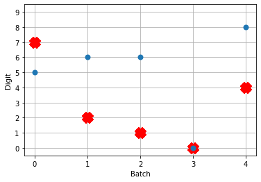
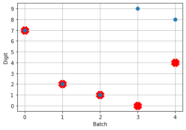
Next, we can load our trained parameters, call the sim.predict function and plot the results:
n_test = 5
with nengo_dl.Simulator(net, seed=0) as sim:
    sim.load_params(params_file)
    data = sim.predict({nengo_input: test_images[:n_test]})

# plot the answer in a big red x
plt.plot(test_labels[:n_test].squeeze(), 'rx', mew=15)
# data[nengo_output].shape = (images, timesteps, n_outputs)
# plot predicted digit from network output on the last time step
plt.plot(np.argmax(data[nengo_output][:, -1], axis=1), 'o', mew=2)

NengoDL inherently accounts for time in its simulations and so the data all needs to be formatted as (n_batches, n_timesteps, n_inputs). In this case everything is using standard rate mode neurons with no internal states that change over time, so simulating the network over time will generate the same output at every time step. When we move to spiking neurons, however, effects of temporal dynamics will be visible.
Convert to spiking neurons
To convert our network to spiking neurons, all we have to do is change the neuron activation function that we map to in the converter when we’re generating the net:
converter = nengo_dl.Converter(
    model,
    swap_activations={tf.nn.relu: nengo.SpikingRectifiedLinear()},
)
net = converter.net
nengo_input = converter.inputs[input]
nengo_output = converter.outputs[dense1]

with nengo_dl.Simulator(net) as sim:
    sim.load_params("mnist_params")
    data = sim.predict({nengo_input: test_images[:n_test]})
So the process is that we create the model using Keras once. Then we can use a NengoDL Converter to create a Nengo network that can be simulated and trained. We save the parameters after training, and now we can use another Converter to create another instance of the network that uses SpikingRectifiedLinear neurons as the activation function. We can then load in the trained parameters that we got from simulating the standard RectifiedLinear rate mode activation function.
The reason that we don’t do the training with the SpikingRectifiedLinear activation function is because of its discontinuities, which cause errors when trying to calculate the derivative in backprop.
So! What kind of results do we get now that we’ve converted into spiking neurons?

Not great! Why is this happening? Good question. It seems like what’s happening is the network is really convinced everything is 5. To investigate, we’re going to need to look at the neural activity.
Plotting the neural activity over time
To be able to see the activity of the neurons, we’re going to need 1) a reference to the ensemble of neurons we’re interested in monitoring, and 2) a Probe to track the activity of those neurons during simulation. This involves changing the network, so we’ll create another converted network and modify it before passing it into our Simulator.
converter = nengo_dl.Converter(
    model,
    swap_activations={tf.nn.relu: nengo.SpikingRectifiedLinear()},
)
net = converter.net

nengo_input = converter.inputs[input]
nengo_output = converter.outputs[dense1]
# get a reference for the neurons that we want to probe
nengo_conv1 = converter.layers[conv1]

# add probe to the network to track the activity of those neurons!
with converter.net as net:
    probe_conv1 = nengo.Probe(nengo_conv1, label='probe_conv1')

with nengo_dl.Simulator(net) as sim:
    sim.load_params("mnist_params")
    data = sim.predict({nengo_input: test_images[:n_test]})
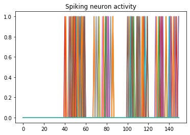
We can use Nengo’s handy rasterplot helper function to plot the activity of the first 3000 neurons:
from nengo.utils.matplotlib import rasterplot
# plot results neural activity from the first n_neurons on the
# first batch (each image is a batch), all time steps
rasterplot(np.arange(n_timesteps), data[probe_conv1][0, :, :n_neurons])
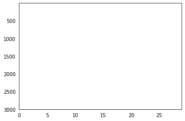
If you have a keen eye and familiar with raster plots, you may notice that there are no spikes. Not a single one! So our network isn’t predicting a 5 for each input, it’s not predicting anything. We’re just getting 5 as output from a learned bias term. Bummer.
Let’s go back and see what kind of output our rate mode neurons are giving us, maybe that can help explain what’s going on. We can’t use a raster plot, because there are no spikes, but we can use a regular plot.
converter = nengo_dl.Converter(
model,
swap_activations={tf.nn.relu: nengo.RectifiedLinear()},
)
net = converter.net
nengo_input = converter.inputs[input]
nengo_output = converter.outputs[dense1]
nengo_conv1 = converter.layers[conv1]
with net:
probe_conv1 = nengo.Probe(nengo_conv1)
with nengo_dl.Simulator(net) as sim:
sim.load_params("mnist_params")
data = sim.predict({nengo_input: test_images[:n_test]})
n_neurons = 5000
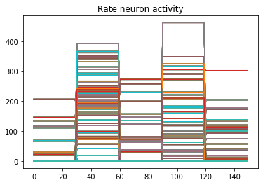
print('Max value: ', np.max(data[probe_conv1].flatten()))
# plot activity of first 5000 neurons, all inputs, all time steps
# we reshape the data so it's (n_batches * n_timesteps, n_neurons)
# for ease of plotting
plt.plot(data[probe_conv1][:, :, :n_neurons].reshape(-1, n_neurons))
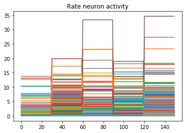
Looking at the rate mode activity of the neurons, we see that the max firing rate is 34.6Hz. That’s about 1 spike every 30 milliseconds. Through an unlucky coincidence we’ve set each image to be presented to the network for 30ms. What could be happening is that neurons are building up to the point of spiking, but the input is switched before they actually spike. To test this, let’s change the number of time steps each image is presented to 100ms, and rerun our spiking simulator.
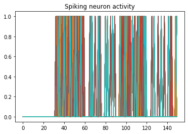
We’ll also switch over to plotting spiking activity the same way as the rate neurons for consistency (and because it’s easier to see if neurons are spiking or not when there’s really sparse activity). One thing you may note below is that I’m plotting activity * dt, instead of just activity like in the rate neuron case. Whenever there’s a spike in Nengo, it’s recorded as 1/dt so that it integrates to 1. Multiplying the probe output by dt means that we see a 1 when there’s one spike per time step, a 2 when there’s two spikes per time step, etc. It just makes it a bit easier to read.
print('Max value: ', np.max(data[probe_conv1].flatten() * dt))
print(data[probe_conv1][:,:,:n_neurons].shape)
plt.plot(data[probe_conv1][:, :, :n_neurons].reshape(-1, n_neurons) * dt)
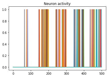
Looking at this plot, we can see a few things. First, whenever an image is presented, there’s a startup period where no spikes occur. Ideally our network will give us some output without having to present input for 50 time steps (the rate network gives us output after 1 time step!) We can address this by increasing the firing rates of the neurons in our network. We’ll come back to this.
Second, even now that we’re getting spikes, the predictions for each image are very poor. Why is that happening? Let’s look at the network output over time when we feed in the first test image:
From this plot it looks like there’s not a clear prediction so much as a bunch of noise. One factor that can contribute to this is that the way things are set up right now, when a neuron spikes that information is only processed by the receiving side for 1 time step. Anthropomorphizing our network, you can think of the output layer as receiving input along the lines of “nothing … nothing … nothing … IT’S A 5! … maybe a 2? … maybe a 3? … IT’S A 5! ..” etc.
It would be useful for us to do a bit of averaging over time. Enter: synapses!
Using synapses to smooth the output of a spiking network
Synapses can come in many forms. The default form in Nengo is a low-pass filter. What this does for us is let the post-synaptic neuron (i.e. the neuron that we’re sending information to) do a bit of integration of the information that is being sent to it. So in the above example the output layer would be receiving input like “nothing … nothing … nothing … looking like a 5 … IT’S A 5! … it’s a 5! … it’s probably a 5 but maybe also a 2 or 3 … IT’S A 5! … ” etc.
Likely it will be more useful for understanding to see the actual network output over time with different low-pass filters applied rather than reading strained metaphors.
To make apply a low-pass filter synapse to all of the connections in our network is easy enough, we just add another modification to the network before passing it into the Simulator:
converter = nengo_dl.Converter(
    model,
    swap_activations={tf.nn.relu: nengo.SpikingRectifiedLinear()},
)
net = converter.net

nengo_input = converter.inputs[input]
nengo_output = converter.outputs[dense1]
nengo_conv1 = converter.layers[conv1]

with net:
    probe_conv1 = nengo.Probe(nengo_conv1)

# set a low-pass filter value on all synapses in the network
for conn in net.all_connections:
    conn.synapse = 0.001

with nengo_dl.Simulator(net) as sim:
    sim.load_params("mnist_params")
    data = sim.predict({nengo_input: test_images[:n_test]})
And here are the results we get for different low-pass filter time constants:
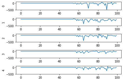

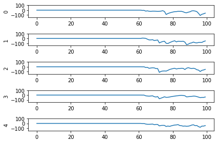

As the time constant on the low-pass filter increases, we can see the output of the network starts smoothing out. It’s important to recognize that there are a few things going on though when we filter values on all of the synapses of the network. The first is that we’re no longer sending sharp spikes between layers, we’re now passing along filtered spikes. The larger the time constant on the filter, the more spread out and smoother the signal will be.
As a result of this: If sending a spike from neuron A to neuron B used to cause neuron B to spike immediately when there was no synaptic filter, that may no longer be the case. It may now take several spikes from neuron A, all close together in time, for neuron B to now spike.
Another thing we want to consider is that we’ve applied a synaptic filter at every layer, so the dynamics of the entire network have changed. Very often you’ll want to be more surgical with the synapses you create, leaving some connections with no synapse and some with large filters to get the best performance out of your network. Currently the way to do this is to print out net.all_connections, find the connections of interest, and then index in specific values. When we print out net.all_connections for this network, we get:
[<Connection at 0x7fd8ac65e4a8 from <Node "conv2d.0.bias"> to <Node (unlabeled) at 0x7fd8ac65ee48>>,
<Connection at 0x7fd969a06b70 from <Node (unlabeled) at 0x7fd8ac65ee48> to <Neurons of <Ensemble "conv2d.0">>>,
<Connection at 0x7fd969a06390 from <Node "input_1"> to <Neurons of <Ensemble "conv2d.0">>>,
<Connection at 0x7fd8afc41470 from <Node "dense.0.bias"> to <Node "dense.0">>,
<Connection at 0x7fd8afc41588 from <Neurons of <Ensemble "conv2d.0">> to <Node "dense.0">>]
The connections of interest for us are from input_1 to conv2d.0, and from conv2d.0 to dense.0. These are the connections the input signals for the network are flowing through, the rest of the connections are just to send in trained bias values to each layer. We can set the synapse value for these connections specifically with the following:
synapses = [None, None, 0.001, None, 0.001]
for conn, synapse in zip(net.all_connections, synapses):
    conn.synapse = synapse
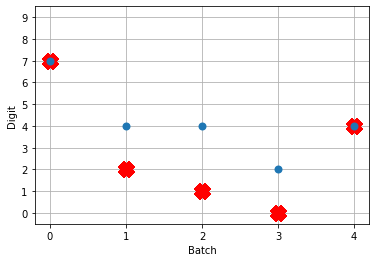
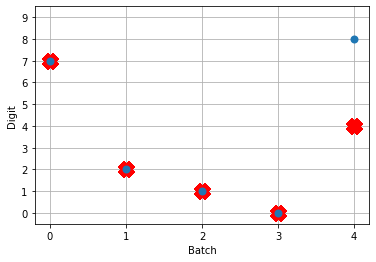
In this case, with just some playing around with different values I wasn’t able to find any synapse values that got better performance than 4/5. But in general being able to set specific synapse values in a spiking neural network is important and you should be aware of how to do it to get the best performance out of your network.
So setting the synapses is able to improve the performance of the network. We’re still taking 100ms to generate output though, and only getting 4/5 of the test set correct. Let’s go back now to the first issue we identified and look at increasing the firing rates of the neurons.
Increasing the firing rates of neurons in the network
There are a few ways to go about this. The first is a somewhat cheeky method that works best for rectified linear (ReLU) neurons, and the second is a more general method that adjusts how training is performed.
Scaling ReLU firing rates
Because we’re using rectified linear neurons in this model, one trick that we can use to increase the firing rates without affecting the functionality of the network is by using a scaling term to multiply the input and divide the output of each neuron. This scaling can work because the rectified linear neuron model is linear in its activation function.
The result of this scaling is more frequent spiking at a lower amplitude. We can implement this using the Nengo DL Converter with the scale_firing_rates keyword:
converter = nengo_dl.Converter(
    model,
    swap_activations={tf.nn.relu: nengo.SpikingRectifiedLinear()},
    scale_firing_rates=gain_scale,
)
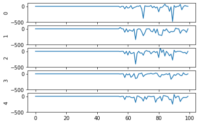
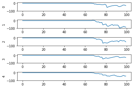
Let’s look at the network output and neural activity plots for gain_scale values of [5, 20, 50].


One thing that’s apparent is as the firing rates go up, the performance of the network gets better. You may notice that for the first image (first 30 time steps) in the spiking activity plots there’s no response. Don’t read too much into that; I’m plotting a random subset of neurons and it just happens that none of them respond to the first image. If I was to plot the activity of all of the neurons we’d see spikes everywhere.
You may also notice that when gain_scale = 50 we’re even getting some neurons that are spiking 2 times per time step. That will happen when the input to the neuron causes the internal state to jump up to twice the threshold for spiking for that neuron. This is not unexpected behaviour.
Using this scale_firing_rates keyword in the Converter is one way to get the performance of our coverted spiking networks to match the performance of rate neuron networks. However, it mainly a trick useful for us for ReLUs (and any other linear activation functions). It would behoove us to figure out another method that will work as well for nonlinear activation functions as well.
Adding a firing rate term to the cost function during training
Let’s go back to the training the network step. Another way to bring the firing rates up is by adding a term to the cost function that will penalize any firing rates outside of some desired range. There are a ton of ways to go about this with different kinds of cost functions. I’m just going to present one cost function term that works for this situation and note that you can build this cost function a whole bunch of different ways. Here’s one:
def put_in_range(x, y, weight=100.0, min=200, max=300):
    index_greater = (y > max)  # find neurons firing faster
    index_lesser = (y < min)  # find neurons firing slower
    error = tf.reduce_sum(y[index_greater] - max) + tf.reduce_sum(min - y[index_lesser])
    return weight * error
The weight parameter lets us set the relative importance of the firing rates cost function term relative to the classification accuracy cost function term. To use this term we need to make a couple of adjustments to our code for training the network:
converter = nengo_dl.Converter(
    model,
    swap_activations={tf.nn.relu: nengo.RectifiedLinear()},
)
net = converter.net

nengo_input = converter.inputs[input]
nengo_output = converter.outputs[dense1]

nengo_conv1 = converter.layers[conv1]
with converter.net as net:
    probe_conv1 = nengo.Probe(nengo_conv1, label='probe_conv1')

# run training
with nengo_dl.Simulator(net) as sim:
    sim.compile(
        optimizer=tf.optimizers.RMSprop(0.001),
        loss={
            nengo_output: tf.losses.SparseCategoricalCrossentropy(from_logits=True),
            probe_conv1: put_in_range,
        }
    )
    sim.fit(
        train_images,
        {nengo_output: train_labels,
         probe_conv1: np.zeros(train_labels.shape)},
        epochs=10)
Mainly what’s been added in this code is our new loss function put_in_range and in the sim.compile call we added probe_conv1: put_in_range to the loss dictionary. This tells Nengo DL to use the put_in_range cost function on the output from probe_conv1, which will be the firing rates of the convolutional layer of neurons in the network.
We also had to add in probe_conv1: np.zeros(train_labels.shape) to the input dictionary in the sim.fit function call. The array specified here is used as the x input to the put_in_range cost function, but since we defined the put_in_range function to be fully determined based only on y (which is the output from probe_conv1) it doesn’t matter what values we pass in there. So I pass in an array of zeros.
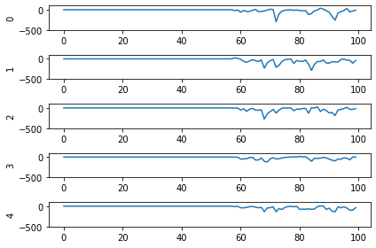
Now when we run the training and prediction in rate mode, the output we get looks like

And we can see that we’re still getting the same performance, but now the firing rates of the neurons are much higher. Let’s see what happens when we convert to spiking neurons now!

Hey, that’s looking much better! This of course is only looking at 5 test images and you’ll want to go through and calculate proper performance statistics using a full test set, but it’s a good start.
Conclusions
This post has looked at how to take a model that you built in Keras and convert it over to a spiking neural network using Nengo DL’s Converter function. This was a simple model, but hopefully it gets across that the conversion to spikes can be an iterative process, and you now have a better sense of some of the steps that you can take to investigate and debug spiking neural network behaviour! In general when tuning your network you’ll use a mix of the different methods we’ve gone through here, depending on the exact situation.
Again a reminder that all of the code for this can be found up on my GitHub.
Also! It’s very much worth checking out the Nengo DL documentation and other examples that they have there. There’s a great introduction for users coming from TensorFlow over to Nengo, and other examples showing how you can integrate non-spiking networks with spiking networks, as well as other ways to optimizing your spiking neural networks. If you start playing around with Nengo and have more questions, please feel free to ask in comments below or even better go to the Nengo forums!
