Dynamic movement primitive

May 13 2016

Dynamic movement primitive, motor control, Python, Robotics

Dynamic movement primitives part 4: Avoiding obstacles – update

Edit: Previously I posted this blog post on incorporating obstacle avoidance, but after a recent comment on the code I started going through it again and found a whole bunch of issues. Enough so that I’ve recoded things and I’m going to repost it now with working examples and a description of the changes I made to get it going. The edited sections will be separated out with these nice horizontal lines. If you’re just looking for the example code, you can find it up on my pydmps repo, here.

Alright. Previously I’d mentioned in one of these posts that DMPs are awesome for generalization and extension, and one of the ways that they can be extended is by incorporating obstacle avoidance dynamics. Recently I wanted to implement these dynamics, and after a bit of finagling I got it working, and so that’s going to be the subject of this post.

There are a few papers that talk about this, but the one we’re going to use is Biologically-inspired dynamical systems for movement generation: automatic real-time goal adaptation and obstacle avoidance by Hoffmann and others from Stefan Schaal’s lab. This is actually the second paper talking about obstacle avoidance and DMPs, and this is a good chance to stress one of the most important rules of implementing algorithms discussed in papers: collect at least 2-3 papers detailing the algorithm (if possible) before attempting to implement it. There are several reasons for this, the first and most important is that there are likely some typos in the equations of one paper, by comparing across a few papers it’s easier to identify trickier parts, after which thinking through what the correct form should be is usually straightforward. Secondly, often equations are updated with simplified notation or dynamics in later papers, and you can save yourself a lot of headaches in trying to understand them just by reading a later iteration. I recklessly disregarded this advice and started implementation using a single, earlier paper which had a few key typos in the equations and spent a lot of time tracking down the problem. This is just a peril inherent in any paper that doesn’t provide tested code, which is almost all, sadface.

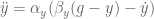
OK, now on to the dynamics. Fortunately, I can just reference the previous posts on DMPs here and don’t have to spend any time discussing how we arrive at the DMP dynamics (for a 2D system):

$\ddot{\textbf{y}} = \alpha_y (\beta_y( \textbf{g} - \textbf{y}) - \dot{\textbf{y}}) + \textbf{f},$

where $\alpha_y$ and $\beta_y$ are gain terms, $\textbf{g}$ is the goal state, $\textbf{y}$ is the system state, $\dot{\textbf{y}}$ is the system velocity, and $\textbf{f}$ is the forcing function.
As mentioned, DMPs are awesome because now to add obstacle avoidance all we have to do is add another term

$\ddot{\textbf{y}} = \alpha_y (\beta_y( \textbf{g} - \textbf{y}) - \dot{\textbf{y}}) + \textbf{f} + \textbf{p}(\textbf{y}, \dot{\textbf{y}}),$

where $\textbf{p}(\textbf{y}, \dot{\textbf{y}})$ implements the obstacle avoidance dynamics, and is a function of the DMP state and velocity. Now then, the question is what are these dynamics exactly?

Obstacle avoidance dynamics

It turns out that there is a paper by Fajen and Warren that details an algorithm that mimics human obstacle avoidance. The idea is that you calculate the angle between your current velocity and the direction to the obstacle, and then turn away from the obstacle. The angle between current velocity and direction to the obstacle is referred to as the steering angle, denoted $\varphi$ , here’s a picture of it:

So, given some $\varphi$ value, we want to specify how much to change our steering direction, $\dot{\varphi}$ , as in the figure below:

If we’re on track to hit the object (i.e. $\varphi$ is near 0) then we steer away hard, and then make your change in direction less and less as the angle between your heading (velocity) and the object is larger and larger. Formally, define $\dot{\varphi}$ as

$\dot{\varphi} = \gamma \;\varphi \;\textrm{exp}(-\beta | \varphi |),$

where $\gamma$ and $\beta$ are constants, which are specified as $1000$ and $\frac{20}{\pi}$ in the paper, respectively.

Edit: OK this all sounds great, but quickly you run into issues here. The first is how do we calculate $\varphi$ ? In the paper I was going off of they used a dot product between the $\dot{\textbf{y}}$ vector and the $\textbf{o} - \textbf{y}$ vector to get the cosine of the angle, and then use np.arccos to get the angle from that. There is a big problem with this here, however, that’s kind of subtle: You will never get a negative angle when you calculate this, which, of course. That’s not how np.arccos works, but it is still what we need so we will be able to tell if we should be turning left or right to avoid this object!

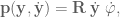
So we need to use a different way of calculating the angle, one that tells us if the object is in a + or – angle relative to the way we’re headed. To calculate an angle that will give us + or -, we’re going to use the np.arctan2 function.

We want to center things around the way we’re headed, so first we calculate the angle of the direction vector, $\dot{\textbf{y}}$ . Then we create a rotation vector, R_dy to rotate the vector describing the direction of the object. This shifts things around so that if we’re moving straight towards the object it’s at 0 degrees, if we’re headed directly away from it, it’s at 180 degrees, etc. Once we have that vector, nooowwww we can find the angle of the direction of the object and that’s what we’re going to use for phi. Huzzah!

# get the angle we're heading in
phi_dy = -np.arctan2(dy[1], dy[0]) 
R_dy = np.array([[np.cos(phi_dy), -np.sin(phi_dy)],
                 [np.sin(phi_dy), np.cos(phi_dy)]])
# calculate vector to object relative to body
obj_vec = obstacle - y
# rotate it by the direction we're going 
obj_vec = np.dot(R_dy, obj_vec)
# calculate the angle of obj relative to the direction we're going
phi = np.arctan2(obj_vec[1], obj_vec[0])

This $\dot{\varphi}$ term can be thought of as a weighting, telling us how much we need to rotate based on how close we are to running into the object. To calculate how we should rotate we’re going to calculate the angle orthonormal to our current velocity, then weight it by the distance between the object and our current state on each axis. Formally, this is written:

$\textbf{R} \; \dot{\textbf{y}},$

where $\textbf{R}$ is the axis $(\textbf{o} - \textbf{y}) \times \dot{\textbf{y}}$ rotated 90 degrees (the $\times$ denoting outer product here). The way I’ve been thinking about this is basically taking your velocity vector, $\dot{\textbf{y}}$ , and rotating it 90 degrees. Then we use this rotated vector as a row vector, and weight the top row by the distance between the object and the system along the $x$ axis, and the bottom row by the difference along the $\textbf{y}$ axis. So in the end we’re calculating the angle that rotates our velocity vector 90 degrees, weighted by distance to the object along each axis.

So that whole thing takes into account absolute distance to object along each axis, but that’s not quite enough. We also need to throw in $\dot{\varphi}$ , which looks at the current angle. What this does is basically look at ‘hey are we going to hit this object?’, if you are on course then make a big turn and if you’re not then turn less or not at all. Phew.

OK so all in all this whole term is written out

$\textbf{p}(\textbf{y}, \dot{\textbf{y}}) = \textbf{R} \; \dot{\textbf{y}} \; \dot{\varphi},$

and that’s what we add in to the system acceleration. And now our DMP can avoid obstacles! How cool is that?

Super compact, straight-forward to add, here’s the code:

Edit: OK, so not suuuper compact. I’ve also added in another couple checks. The big one is “Is this obstacle between us and the target or not?”. So I calculate the Euclidean distance to the goal and the obstacle, and if the obstacle is further away then the goal, set the avoidance signal to zero (performed at the end of the if)! This took care of a few weird errors where you would get a big deviation in the trajectory if it saw an obstacle past the goal, because it was planning on avoiding it, but then was pulled back in to the goal before the obstacle anyways so it was a pointless exercise. The other check added in is just to make sure you only add in obstacle avoidance if the system is actually moving. Finally, I also changed the $\gamma = 100$ instead of $1000$ .

def avoid_obstacles(y, dy, goal):
    p = np.zeros(2)
 
    for obstacle in obstacles:
        # based on (Hoffmann, 2009)

        # if we're moving
        if np.linalg.norm(dy) > 1e-5:

            # get the angle we're heading in
            phi_dy = -np.arctan2(dy[1], dy[0]) 
            R_dy = np.array([[np.cos(phi_dy), -np.sin(phi_dy)],
                             [np.sin(phi_dy), np.cos(phi_dy)]])
            # calculate vector to object relative to body
            obj_vec = obstacle - y
            # rotate it by the direction we're going 
            obj_vec = np.dot(R_dy, obj_vec)
            # calculate the angle of obj relative to the direction we're going
            phi = np.arctan2(obj_vec[1], obj_vec[0])

            dphi = gamma * phi * np.exp(-beta * abs(phi))
            R = np.dot(R_halfpi, np.outer(obstacle - y, dy))
            pval = -np.nan_to_num(np.dot(R, dy) * dphi)

            # check to see if the distance to the obstacle is further than 
            # the distance to the target, if it is, ignore the obstacle
            if np.linalg.norm(obj_vec) > np.linalg.norm(goal - y):
                pval = 0

            p += pval
    return p

And that’s it! Just add this method in to your DMP system and call avoid_obstacles at every timestep, and add it in to your DMP acceleration.

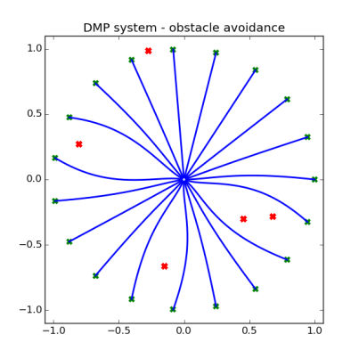
You hopefully noticed in the code that this is set up for multiple obstacles, and that all that that entailed was simply adding the p value generated by each individual obstacle. It’s super easy! Here’s a very basic graphic showing how the DMP system can avoid obstacles:

So here there’s just a basic attractor system (DMP without a forcing function) trying to move from the center position to 8 targets around the unit circle (which are highlighted in red), and there are 4 obstacles that I’ve thrown onto the field (black x’s). As you can see, the system successfully steers way clear of the obstacles while moving towards the target!

We must all use this power wisely.

Edit: Making the power yours is now easier than ever! You can check out this code at my pydmps GitHub repo. Clone the repo and after you python setup.py develop, change directories into the examples folder and run the avoid_obstacles.py file. It will randomly generate 5 targets in the environment and perform 20 movements, giving you something looking like this:

Tagged control, Dynamic movement primitives, operational space control, robot control, robotics

Mar 07 2014

11 Comments

Dynamic movement primitive, math, motor control, PID control, Python, Robotics

Dynamic movement primitives part 3: Rhythmic movements

So far we’ve looked at using DMPs for discrete movements, but as I briefly mentioned it’s also possible to use them to perform rhythmic movements. In this post we’re going to look at the implementation of rhythmic DMPs and see exactly how it’s done. It’s actually pretty straightforward, which is always nich. We’ll go through everything that has to change and then see a couple of different applications of rhythmic DMPs. Again, all the code for the DMPs and arm control implementations can be found up on my Github.

Obtaining consistent and repeatable basis function activation

We’ll start with the canonical system. In the discrete case our canonical system (which drives the activation of the basis functions) decayed from $1$ to $0$ and then we were all done. In the rhythmic case we want our system to repeat indefinitely, so we need a reliable way of continuously activating the basis functions in the same order. One function that may come to mind that reliably repeats is the cosine function. But how to use the cosine function, exactly?

The idea is that we’ll lay out our basis functions in the range from $0$ to $2\pi$ , and we’ll set the canonical system to be ever increasing linearly. Then we’ll use the difference between the canonical system state and each of the center points as the value we pass in to our cosine function. Because the cosine function repeats at $2\pi$ we’ll get a nice repeating spread of basis function activations. We’ll then throw these values through our Gaussian equation (with the gain and bias terms) and we’ll be done! Here’s the equation:

$\psi = \textrm{exp}(h * \textrm{cos}(x - c) - 1),$
where $x$ is the state of the canonical system, $c$ is the basis function center point, and $h$ is a gain term controlling the variance of the Gaussian. And here’s a picture of the activations of three basis functions with centers spread out evenly between $0$ and $2\pi$ :

Here’s a picture of the basis function activations on a longer time scale:

As long as our canonical system increases at a steady pace the basis functions will continue to activate in a reliable and repeatable way. As mentioned, to get the canonical system to increase at a steady pace we simply give it linear dynamics:

$\dot{x} = 1$
The placement of the center points of the rhythmic system is a lot easier than in the discrete case because the rhythmic canonical system dynamics are linear.

Other differences between discrete and rhythmic

In the actual implementation of the rhythmic system there are a couple of other differences that you need to be aware of. The first is that there is no diminishing term in the rhythmic system, whereas there is in the discrete case.

The second is how to go about establishing goal states when imitating an path. We’re going to assume that whatever path is passed in to us is going to be a rhythmic pattern, and then goal state is going to be set as the center point of the desired trajectory. So for rhythmic systems the ‘goal’ is actually more like a center point for the trajectory.

And that’s pretty much it! If you look through the code that I have up for the rhythmic DMP subclass you’ll see that only a handful of functions needed to be redefined, the rest is the same! Well that’s great, let’s look at some applications.

Example

I was thinking of different examples that would be interesting to see of the rhythmic DMPs, and after a little consideration the most obvious application of rhythmic DMPs is really to a system that does something like walking. In the spinal cord of animals there are circuits which are known as central pattern generators (CPGs), and when stimulated these have been shown to generate rhythmic, repeated movements (as described in Principles of rhythmic motor pattern generation and other papers). Let’s go ahead and build our own CPG here using DMPs. I don’t have a simulation of a set of legs, however, so instead we’ll look at getting a single 3-link arm to reproduce a pattern of behaviour that you’d expect in a leg that is walking.

To do this, I’m going to need to specify the trajectories for the three joints of the arm, and I’ll be controlling the system in joint space, using the generalized coordinates controller, rather than the operational space controller used in the discrete DMP examples for controlling the end-effector position. So that’s one thing. Another thing is that I’m going to need the kinematics of leg joints during motion. After a quick search of the web I found this presentation from Simon Fraser University which has the following images:

Which is some very useful information! I just need to transfer this into a Numpy vector that I can feed into the system and convert degrees to radians and we should be good to go! To get the information out of the graph, use your favorite data stripper, I used http://arohatgi.info/WebPlotDigitizer/app/.

I also had to do a bit of a shuffle with the trajectories provided to make it look right on the arm. The hip to shoulder joint maps fine, but for the knee to elbow the flexion and extension are reversed, and for the wrist to foot the $0$ angle for the foot is straight out. Once those have been accounted for, though, everything works great. Here is an animation of a single leg walking along, if you use your imagination you can just picture a happy-go-lucky torso attached to this leg whistling while he gets his very human-like gait on:

And there you go! It’s neat how straightforward that was, once you have the data of the system you want to model. It shows the power of DMPs for coordinating multiple degrees of freedom quickly and easily. Also something that’s worth pointing out once again is that this is a force based controller. We were able to go from a kinematic description of the movement we wanted to a reliable system generating torques. It’s another good example of the dexterity of dynamic movement primitives.

You can see the code for everything here up online on my github control repo on the walking_demo branch. To run the code you should run:

python run.py

If you have any questions or trouble running the code please contact me.

Tagged control theory, PD control, rhythmic dynamic movement primitives, walking

Dec 05 2013

30 Comments

Dynamic movement primitive, motor control, Operational space control, PID control, programming, Python, Robotics

Dynamic movement primitives part 2: Controlling end-effector trajectories

The dynamic movement primitive (DMP) framework was designed for trajectory control. It so happens that in previous posts we’ve built up to having several arm simulations that are ripe for throwing a trajectory controller on top, and that’s what we’ll do in this post. The system that we will be controlling here is the 3 link arm model with an operational space controller (OSC) that translates end-effector forces into joint torques. 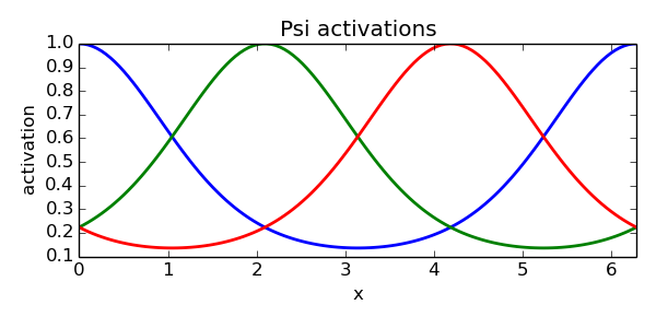The DMPs here will be controlling the $(x,y)$ trajectory of the hand, and the OSC will take care of turning the desired hand forces into torques that can be applied to the arm. All of the code used to generate the animations throughout this post can of course be found up on my github (to run play around with variants of python run.py arm3 dmp write).

Controlling a 3 link arm with DMPs
We have our 3 link arm and its OSC controller; this whole setup we’ll collectively refer to as ‘the plant’ throughout this post. We are going to pass in some $(x,y)$ force signal to the plant, and the plant will carry it out. Additionally we’ll get a feedback signal with the $(x,y)$ position of the hand. At the same time, we also have a DMP system that’s doing its own thing, tracing out a desired trajectory in $(x,y)$ space. We have to tie these two systems together.

To do this is easy, we’ll generate the control signal for the plant from our DMP system simply by measuring the difference between the state of our DMP system and the plant state, use that to drive the plant to the state of the DMP system. Formally,

$u = k_p(y_{\textrm{DMP}} - y)$

where $y_{\textrm{DMP}}$ is the state of the DMP system, $y$ is the state of the plant, and $k_p$ and is the position error gain term.

Once we have this, we just go ahead and step our DMP system forward and make sure the gain values on the control signal are high enough that the plant follows the DMP’s trajectory. And that’s pretty much it, just run the DMP system to the end of the trajectory and then stop your simulation.

To give a demonstration of DMP control I’ve set up the DMP system to follow the same number trajectories that the SPAUN arm followed. As you can see the combination of DMPs and operational space control is much more effective than my previous implementation.

Incorporating system feedback

One of the issues in implementing the control above is that we have to be careful about how quickly the DMP trajectory moves, because while the DMP system isn’t constrained by any physical dynamics, the plant is. Depending on the size of the movement the DMP trajectory may be moving a foot a second or an inch a second. You can see above that the arm doesn’t fully draw out the desired trajectories in places where the DMP system moved too quickly in and out and sharp corners. The only way to remedy this without feedback is to have the DMP system move more slowly throughout the entire trajectory. What would be nice, instead, would be to just say ‘go as fast as you can, as long as the plant state is within some threshold distance of you’, and this is where system feedback comes in.

It’s actually very straightforward to implement this using system feedback: If the plant state drifts away from the state of the DMPs, slow down the execution speed of the DMP to allow the plant time to catch up. The do this we just have to multiply the DMP timestep $dt$ by a new term:

$1 / (1 + \alpha_{\textrm{err}}(y_{\textrm{plant}} - y_{\textrm{DMP}}))$ .

All this new term does is slow down the canonical system when there’s an error, you can think of it as a scaling on the time step. Additionally, the sensitivity of this term can be modulated the scaling term $\alpha_{\textrm{err}}$ on the difference between the plant and DMP states.

We can get an idea of how this affects the system by looking at the dynamics of the canonical system when an error term is introduced mid-run:

When the error is introduced the dynamics of the system slow down, great! Lets look at an example comparing execution with and without this feedback term. Here’s the system drawing the number 3 without any feedback incorporation:

and here’s the system drawing the number 3 with the feedback term included:

These two examples are a pretty good case for including the feedback term into your DMP system. You can still see in the second case that the specified trajectory isn’t traced out exactly, but if that’s what you’re shooting for you can just crank up the $\alpha_{\textrm{err}}$ to make the DMP timestep really slow down whenever the DMP gets ahead of the plant at all.

Interpolating trajectories for imitation

When imitating trajectories there can be some issues with having enough sample points and how to fit them to the canonical system’s timeframe, they’re not difficult to get around but I thought I would go over what I did here. The approach I took was to always run the canonical system for 1 second, and whenever a trajectory is passed in that should be imitated to scale the x-axis of the trajectory such that it’s between 0 and 1. Then I shove it into an interpolator and use the resulting function to generate an abundance of nicely spaced sample points for the DMP imitator to match. Here’s the code for that:

# generate function to interpolate the desired trajectory
import scipy.interpolate

path = np.zeros((self.dmps, self.timesteps))
x = np.linspace(0, self.cs.run_time, y_des.shape[1])

for d in range(self.dmps):

# create interpolation function
path_gen = scipy.interpolate.interp1d(x, y_des[d])

# create evenly spaced sample points of desired trajectory
for t in range(self.timesteps):
path[d, t] = path_gen(t * self.dt)

y_des = path

Direct trajectory control vs DMP based control

Now, using the above described interpolation function we can just directly use its output to guide our system. And, in fact, when we do this we get very precise control of the end-effector, more precise than the DMP control, as it happens. The reason for this is because our DMP system is approximating the desired trajectory and with a set of basis functions, and some accuracy is being lost in this approximation.

So if we instead use the interpolation function to drive the plant we can get exactly the points that we specified. The times when this comes up especially are when the trajectories that you’re trying to imitate are especially complicated. There are ways to address this with DMPs by placing your basis functions more appropriately, but if you’re just looking for the exact replication of an input trajectory (as often people are) this is a simpler way to go. You can see the execution of this in the trace.py code up on my github. Here’s a comparison of a single word drawn using the interpolation function:

and here’s the same word drawn using a DMP system with 1,000 basis function per DOF:

We can see that just using the interpolation function here gives us the exact path that we specified, where using DMPs we have some error, and this error increases with the size of the desired trajectory. But! That’s for exactly following a given trajectory, which is often not the case. The strength of the DMP framework is that the trajectory is a dynamical system. This lets us do simple things to get really neat performance, like scale the trajectory spatially on the fly simply by changing the goal, rather than rescaling the entire trajectory:

Conclusions

Some basic examples of using DMPs to control the end-effector trajectory of an arm with operational space control were gone over here, and you can see that they work really nicely together. I like when things build like this. We also saw that power of DMPs in this situation is in their generalizability, and not in exact reproduction of a given path. If I have a single complex trajectory that I only want the end-effector to follow once then I’m going to be better off just interpolating that trajectory and feeding the coordinates into the arm controller rather than go through the whole process of setting up the DMPs.

Drawing words, though, is just one basic example of using the DMP framework. It’s a very simple application and really doesn’t do justice to the flexibility and power of DMPs. Other example applications include things like playing ping pong. This is done by creating a desired trajectory showing the robot how to swing a ping pong paddle, and then using a vision system to track the current location of the incoming ping pong ball and changing the target of the movement to compensate dynamically. There’s also some really awesome stuff with object avoidance, that is implemented by adding another term with some simple dynamics to the DMP. Discussed here, basically you just have another system that moves you away from the object with a strength relative to your distance from the object. You can also use DMPs to control gain terms on your PD control signal, which is useful for things like object manipulation.

And of course I haven’t touched on rhythmic DMPs or learning with DMPs at all, and those are both also really interesting topics! But this serves as a decent introduction to the whole area, which has been developed in the Schaal lab over the last decade or so. I recommend further reading with some of these papers if you’re interested, there are a ton of neat ways to apply the DMP framework! And, again, the code for everything here is up on my github in the control and pydmps repositories.

Tagged arm control, control theory, DMPs, Dynamic movement primitives, operational space control, robotics

Nov 16 2013

60 Comments

Dynamic movement primitive, motor control, Robotics

Dynamic movement primitives part 1: The basics

Dynamic movement primitives (DMPs) are a method of trajectory control / planning from Stefan Schaal’s lab. They were presented way back in 2002 in this paper, and then updated in 2013 by Auke Ijspeert in this paper. This work was motivated by the desire to find a way to represent complex motor actions that can be flexibly adjusted without manual parameter tuning or having to worry about instability.

Complex movements have long been thought to be composed of sets of primitive action ‘building blocks’ executed in sequence and \ or in parallel, and DMPs are a proposed mathematical formalization of these primitives. The difference between DMPs and previously proposed building blocks is that each DMP is a nonlinear dynamical system. The basic idea is that you take a dynamical system with well specified, stable behaviour and add another term that makes it follow some interesting trajectory as it goes about its business. There are two kinds of DMPs: discrete and rhythmic. For discrete movements the base system is a point attractor, and for rhythmic movements a limit cycle is used. In this post we’re only going to worry about discrete DMPs, because by the time we get through all the basics this will already be a long post.

Imagine that you have two systems: An imaginary system where you plan trajectories, and a real system where you carry them out. When you use a DMP what you’re doing is planning a trajectory for your real system to follow. A DMP has its own set of dynamics, and by setting up your DMP properly you can get the control signal for your actual system to follow. If our DMP system is planing a path for the hand to follow, then what gets sent to the real system is the set of forces that need to be applied to the hand. It’s up to the real system to take these hand forces and apply them, by converting them down to joint torques or muscle activations (through something like the operation space control framework) or whatever. That’s pretty much all I’ll say here about the real system, what we’re going to focus on here is the DMP system. But keep in mind that the whole DMP framework is for generating a trajectory \ control signal to guide the real system.

I’ve got the code for the basic discrete DMP setup and examples I work through in this post up on my github, so if you want to jump straight to that, there’s the link! You can run test code for each class just by executing that file.

Discrete DMPs

Let’s start out with point attractor dynamics:

$\ddot{y} = \alpha_y ( \beta_y (g - y) - \dot{y})$ ,

where $y$ is our system state, $g$ is the goal, and $\alpha$ and $\beta$ are gain terms. This should look very familiar, it’s a PD control signal, all this is going to do is draw our system to the target. Now what we’ll do is add on a forcing term that will let us modify this trajectory:

$\ddot{y} = \alpha_y ( \beta_y (g - y) - \dot{y}) + f$ .

How to define a nonlinear function $f$ such that you get the desire behaviour is a non-trivial question. The crux of the DMP framework is an additional nonlinear system used to define the forcing function $f$ over time, giving the problem a well defined structure that can be solved in a straight-forward way and easily generalizes. The introduced system is called the canonical dynamical system, is denoted $x$ , and has very simple dynamics:

$\dot{x} = -\alpha_x x$ .

The forcing function $f$ is defined as a function of the canonical system:

$f(x,g) = \frac{\Sigma_{i=1}^N \psi_i w_i}{\Sigma_{i=1}^N \psi_i} x(g - y_0)$ ,

where $y_0$ is the initial position of the system,

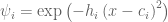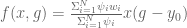
$\psi_i = \textrm{exp}\left( -h_i \left( x - c_i\right)^2 \right)$ ,

and $w_i$ is a weighting for a given basis function $\psi_i$ . You may recognize that the $\psi_i$ equation above defines a Gaussian centered at $c_i$ , where $h_i$ is the variance. So our forcing function is a set of Gaussians that are ‘activated’ as the canonical system $x$ converges to its target. Their weighted summation is normalized, and then multiplied by the $x (g - y_0)$ term, which is both a ‘diminishing’ and spatial scaling term.

Let’s break this down a bit. The canonical system starts at some arbitrary value, throughout this post $x_0 = 1$ , and goes to 0 as time goes to infinity. For right now, let’s pretend that $x$ decays linearly to $0$ . The first main point is that there are some basis functions which are activated as a function of $x$ , this is displayed in the top figure below. As the value of $x$ decreases from 1 to 0, each of the Gaussians are activated (or centered) around different $x$ values. The second thing is that each of these basis functions are also assigned a weight, $w_i$ . These weights are displayed in the lower figure in the bar plot. The output of the forcing function $f$ is then the summation of the activations of these basis functions multiplied by their weight, also displayed in the lower figure below.

The diminishing term
Incorporating the $x$ term into the forcing function guarantees that the contribution of the forcing term goes to zero over time, as the canonical system does. This means that we can sleep easy at night knowing that our system can trace out some crazy path, and regardless will eventually return to its simpler point attractor dynamics and converge to the target.

Spatial scaling
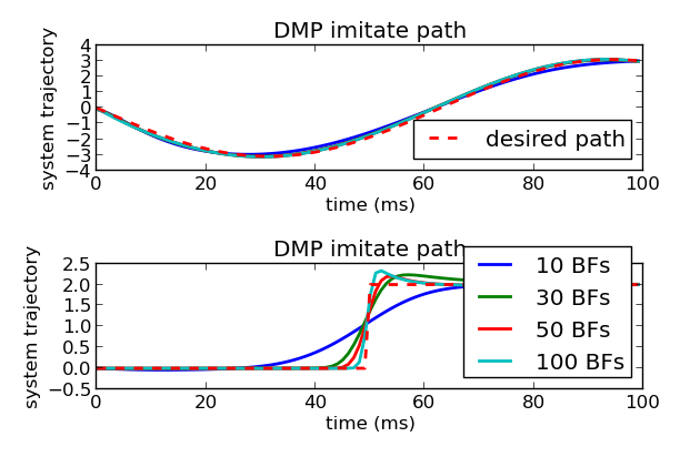
Spatial scaling means that once we’ve set up the system to follow a desired trajectory to a specific goal we would like to be able to move that goal farther away or closer in and get a scaled version of our trajectory. This is what the $(g - y_0)$ term of the forcing function handles, by scaling the activation of each of these basis functions to be relative to the distance to the target, causing the system to cover more or less distance. For example, let’s say that we have a set of discrete DMPs set up to follow a given trajectory:

The goals in this case are 1 and .5, which you can see is where the DMPs end up. Now, we’ve specified everything in this case for these particular goals (1 and .5), but let’s say we’d like to now generalize and get a scaled up version of this trajectory for moving by DMPs to a goal of 2. If we don’t appropriately scale our forcing function, with the $(g - y_0)$ term, then we end up with this:

Basically what’s happened is that for these new goals the same weightings of the basis functions were too weak to get the system to follow or desired trajectory. Once the $(g - y_0)$ term included in the forcing function, however, we get:

which is exactly what we want! Our movements now scale spatially. Awesome.

Spreading basis function centers
Alright, now, unfortunately for us, our canonical system does not converge linearly to the target, as we assumed above. Here’s a comparison of a linear decay vs the exponential decay of actual system:

This is an issue because our basis functions activate dependent on $x$ . If the system was linear then we would be fine and the basis function activations would be well spread out as the system converged to the target. But, with the actual dynamics, $x$ is not a linear function of time. When we plot the basis function activations as a function of time, we see that the majority are activated immediately as $x$ moves quickly at the beginning, and then the activations stretch out as the $x$ slows down at the end:

In the interest of having the basis functions spaced out more evenly through time (so that our forcing function can still move the system along interesting paths as it nears the target, we need to choose our Gaussian center points more shrewdly. If we look at the values of $x$ over time, we can choose the times that we want the Gaussians to be activated, and then work backwards to find the corresponding $x$ value that will give us activation at that time. So, let’s look at a picture:

The red dots are the times we’d like the Gaussians to be centered around, and the blue line is our canonical system $x$ . Following the dotted lines up to the corresponding $x$ values we see what values of $x$ the Gaussians need to be centered around. Additionally, we need to worry a bit about the width of each of the Gaussians, because those activated later will be activated for longer periods of time. To even it out the later basis function widths should be smaller. Through the very nonanalytical method of trial and error I’ve come to calculate the variance as

$h_i = \frac{\#BFs}{c_i}.$

Which reads the variance of basis function $i$ is equal to the number of basis functions divided by the center of that basis function. When we do this, we can now generate centers for our basis functions that are well spaced out:

Temporal scaling

Again, generalizability is one of the really important things that we want out of this system. There are two obvious kinds, temporal and spatial. Spatial scaling we discussed above, in the temporal case we’d like to be able to follow this same trajectory at different speeds. Sometimes quick, sometimes slow, but always tracing out the same path. To do that we’re going to add another term to our system dynamics, $\tau$ , our temporal scaling term. Given that our system dynamics are:

$\ddot{y} = \alpha_y ( \beta_y (g - y) - \dot{y}) + f$ ,
$\dot{x} = -\alpha_x x$ ,

to give us temporal flexibility we can add the $\tau$ term:

$\dot{y}\; +\hspace{-1mm}= \tau \ddot{y}$ ,

$y\; +\hspace{-1mm}= \tau \dot{y}$ ,

$x\; +\hspace{-1mm}= \tau \dot{x}$ ,

and that’s all we have to do! Now to slow down the system you set $\tau$ between 0 and 1, and to speed it up you set $\tau$ greater than 1.

Imitating a desired path

Alright, great. We have a forcing term that can make the system take a weird path as it converges to a target point, and temporal and spatial scalability. How do we set up the system to follow a path that we specify? That would be ideal, to show the system the path to follow, and have it be able to work backwards and figure out the forces and then be able to generate that trajectory whenever we want. This ends up being a pretty straight forward process.

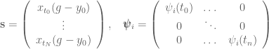
We have control over the forcing term, which affects the system acceleration. So we first need to take our desired trajectory, $\textbf{y}_d$ (where bold denotes a vector, in this case the time series of desired points in the trajectory), and differentiate it twice to get the accelerations:

$\ddot{\textbf{y}}_d = \frac{\partial}{\partial t} \dot{\textbf{y}}_d = \frac{\partial}{\partial t} \frac{\partial}{\partial t} \textbf{y}_d$ .

Once we have the desired acceleration trajectory, we need to remove the effect of the base point attractor system. We have the equation above for exactly what the acceleration induced by the point attractor system at each point in time is:

$\ddot{y} = \alpha_y ( \beta_y (g - y) - \dot{y})$ ,

so then to calculate what the forcing term needs to be generate this trajectory we have:

$\textbf{f}_d = \ddot{\textbf{y}}_d - \alpha_y ( \beta_y (g - \textbf{y}) - \dot{\textbf{y}})$ .

From here we know that the forcing term is comprised of a weighted summation of basis functions which are activated through time, so we can use an optimization technique like locally weighted regression to choose the weights over our basis functions such that the forcing function matches the desired trajectory $\textbf{f}_d$ . In locally weighted regression sets up to minimize:

$\Sigma_t \psi_i(t)(f_d(t) - w_i (x(t) (g - y_0)))^2$

and the solution (which I won’t derive here, but is worked through in Schaal’s 1998 paper ) is

$w_i = \frac{\textbf{s}^T \pmb{\psi}_i \textbf{f}_d}{\textbf{s}^T \pmb{\psi}_i \textbf{s}}$ ,

where

$\textbf{s} = \left( \begin{array}{c}x_{t_0}(g - y_0) \\ \vdots \\ x_{t_N}(g - y_0) \end{array} \right), \;\;\; \pmb{\psi}_i = \left( \begin{array}{ccc} \psi_i(t_0) & \dots & 0 \\ 0 & \ddots & 0 \\ 0 & \dots & \psi_i(t_n) \end{array} \right)$

Great! Now we have everything we need to start making some basic discrete DMPs!

Different numbers of basis functions

One of the things you’ll notice right off the bat when imitating paths, is that as the complexity of the trajectory increases, so does the required number of basis functions. For example, below, the system is trying to follow a sine wave and a highly nonlinear piecewise function:

We can see in the second case that although the DMP is never able to exactly reproduce the desired trajectory, the approximation continues to get better as the number of basis functions increases. This kind of slow improvement in certain nonlinear areas is to be expected from how the basis functions are being placed. An even spreading of the centers of the basis functions through time was used, but for imitation there is another method out of Dr. Schaal’s lab that places the basis functions more strategically. Need is determined by the function complexity is in that region, and basis function centers and widths are defined accordingly. In highly nonlinear areas we would expect there to be many narrow basis functions, and in linear areas we would expect fewer basis functions, but ones that are wider. The method is called locally weighted projection regression, which I plan on writing about and applying in a future post!

Conclusions \ thoughts

There’s really a lot of power in this framework, and there are a ton of expansions on this basic setup, including things like incorporating system feedback, spatio-temporal coupling of DMPs, using DMPs for gain control as well as trajectory control, incorporating a cost function and reinforcement learning, identifying action types, and other really exciting stuff.

I deviated from the terminology used in the papers here in a couple of places. First, I didn’t see a reason to reduce the second order systems to two first order systems. When working through it I found it more confusing than helpful, so I left the dynamics as a second order systems. Second, I also moved the $\tau$ term to the right hand side, and that’s just so that it matches the code, it doesn’t really matter. Neither of these were big changes, but in case you’re reading the papers and wondering.

Something that I kind of skirted above is planning along multiple dimensions. It’s actually very simple; the DMP framework simply assigns one DMP per degree of freedom being controlled. But, it’s definitely worth explicitly stating at some point.

I also mentioned this above, but this is a great trajectory control system to throw on top of the previously discussed operational space control framework. With the DMP framework on top to plan robust, generalizable movements, and the OSCs underneath to carry out those commands we can start to get some really neat applications. For use on real systems the incorporation of feedback and spatio-temporal coupling terms is going to be important, so the next post will likely be working through those and then we can start looking at some exciting implementations!

Speaking of implementations, there’s a DMP and canonical system code up on my github, please feel free to explore it, run it, send me questions about it. Whatever. I should also mention that there’s this and a lot more all up and implemented on Stefan Schaal’s lab website.

Tagged Dynamic movement primitives, high-level controller, motor control, robot control, trajectory planning

studywolf

a blog for things I encounter while coding and researching neuroscience, motor control, and learning

Category Archives: Dynamic movement primitive

Dynamic movement primitives part 4: Avoiding obstacles – update

Dynamic movement primitives part 3: Rhythmic movements

Dynamic movement primitives part 2: Controlling end-effector trajectories

Dynamic movement primitives part 1: The basics