And it has for a while, actually. ‘Oh great’, you may be thinking, ‘but I can never afford the Mujoco license, I’m not a tenured professor!’
Well fear not, friends! Mujoco recently became free for all to use! You can now download their public license and be on your merry way. The associated downside is there’s also no more official support from Dr. Emo Todorov for paid subscribers on the forum. This, I’m sure, is unrelated to my barrage of questions over the years (really I’ve only posted 6 times so it actually probably is unrelated…probably).
And ABR Control has all your favorite examples written up for Mujoco! We’ve got the all the classics:
If you’re not familiar with Mujoco, I highly recommend checking it out. What’s extra nice about Mujoco is that all of the simulation information used to compute the forward dynamics is available (we access it using the mujoco-py package through our mujoco interface file), which means our control is exact. For simulators like CoppelliaSim we don’t have access to this information, so we’re calculating the values ourselves, and there’s often a slight discrepancy. With Mujoco, however, if you set up a floating controller you can bet your bottom dollar that arm will float.
The other benefit of Mujoco, of course, is that it’s super fast, and handles contact dynamics well. Great for robotics applications. Also the visualizations are really slick:
The operational space position and orientation controller running with the path planner running with the Jaco2 arm from Kinova model. The red rectangle is the final target, and the blue rectangle is the path planner target.
I’m very excited that the Mujoco license is free, and I encourage everyone to download it and start playing around. It’s by far the best robotics simulator I’ve used, and it runs fast enough that you can use it to calculate everything you need for controlling a physical robot arm as well (which we’ve also done with the above Jaco2 arm)! The Jaco2, UR5, and a simple geometric arm are included in the ABR Control package, and if you want to have your own arm in there you can follow this previous post about how to build your own model.
So you want to use force control to control the orientation of your end-effector, eh? What a noble endeavour. I, too, wished to control the orientation of the end-effector. While the journey was long and arduous, the resulting code is short and quick to implement. All of the code for reproducing the results shown here is up on my GitHub and in the ABR Control repo.
Introduction
There are numerous resources that introduce the topic of orientation control, so I’m not going to do a full rehash here. I will link to resources that I found helpful, but a quick google search will pull up many useful references on the basics.
When describing the orientation of the end-effector there are three different primary methods used: Euler angles, rotation matrices, and quaternions. The Euler angles , and denote roll, pitch, and yaw, respectively. Rotation matrices specify 3 orthogonal unit vectors, and I describe in detail how to calculate them in this post on forward transforms. And quaternions are 4-dimensional vectors used to describe 3 dimensional orientation, which provide stability and require less memory and compute but are more complicated to understand.
Most modern robotics control is done using quaternions because they do not have singularities, and it is straight forward to convert them to other representations. Fun fact: Quaternion trajectories also interpolate nicely, where Euler angles and rotation matrices do not, so they are used in computer graphics to generate a trajectory for an object to follow in orientation space.
While you won’t need a full understanding of quaternions to use the orientation control code, it definitely helps if anything goes wrong. If you are looking to learn about or brush up on quaternions, or even if you’re not but you haven’t seen this resource, you should definitely check out these interactive videos by Grant Sanderson and Ben Eater. They have done an incredible job developing modules to give people an intuition into how quaternions work, and I can’t recommend their work enough. There’s also a non-interactive video version that covers the same material.
In control literature, angular velocity and acceleration are denoted and . It’s important to remember that is denoting a velocity, and not a position, as we work through things or it could take you a lot longer to understand than it otherwise might…
How to generate task-space angular forces
So, if you recall a post long ago on Jacobians, our task-space Jacobian has 6 rows:
In position control, where we’re only concerned about the position of the hand, the angular velocity dimensions are stripped out of the Jacobian so that it’s a 3 x n_joints matrix rather than a 6 x n_joints matrix. So the orientation of the end-effector is not controlled at all. When we did this, we didn’t need to worry or know anything about the form of the angular velocities.
Now that we’re interested in orientation control, however, we will need to learn up (and thank you to Yitao Ding for clarifying this point in comments on the original version of this post). The Jacobian for the orientation describes the rotational velocities around each axis with respect to joint velocities. The rotational velocity of each axis “happens” at the same time. It’s important to note that this is not the same thing as Euler angles, which are applied sequentially.
To generate our task-space angular forces we will have to generate an orientation angle error signal of the appropriate form. To do that, first we’re going to have to get and be able to manipulate the orientation representation of the end-effector and our target.
Transforming orientation between representations
We can get the current end-effector orientation in rotation matrix form quickly, using the transformation matrices for the robot. To get the target end-effector orientation in the examples below we’ll use the VREP remote API, which returns Euler angles.
It’s important to note that Euler angles can come in 12 different formats. You have to know what kind of Euler angles you’re dealing with (e.g. rotate around X then Y then Z, or rotate around X then Y then X, etc) for all of this to work properly. It should be well documented somewhere, for example the VREP API page tells us that it will return angles corresponding to x, y, and then z rotations.
The axes of rotation can be static (extrinsic rotations) or rotating (intrinsic rotations). NOTE: The VREP page says that they rotate around an absolute frame of reference, which I take to mean static, but I believe that’s a typo on their page. If you calculate the orientation of the end-effector of the UR5 using transform matrices, and then convert it to Euler angles with axes='rxyz' you get a match with the displayed Euler angles, but not with axes='sxyz'.
Now we’re going to have to be able to transform between Euler angles, rotation matrices, and quaternions. There are well established methods for doing this, and a bunch of people have coded things up to do it efficiently. Here I use the very handy transformations module from Christoph Gohlke at the University of California. Importantly, when converting to quaternions, don’t forget to normalize the quaternions to unit length.
from abr_control.arms import ur5 as arm
from abr_control.interfaces import VREP
from abr_control.utils import transformations

robot_config = arm.Config()
interface = VREP(robot_config)
interface.connect()

feedback = interface.get_feedback()
# get the end-effector orientation matrix
R_e = robot_config.R('EE', q=feedback['q'])
# calculate the end-effector unit quaternion
q_e = transformations.unit_vector(
    transformations.quaternion_from_matrix(R_e))

# get the target information from VREP
target = np.hstack([
    interface.get_xyz('target'),
    interface.get_orientation('target')])
# calculate the target orientation rotation matrix
R_d = transformations.euler_matrix(
    target[3], target[4], target[5], axes='rxyz')[:3, :3]
# calculate the target orientation unit quaternion
q_d = transformations.unit_vector(
    transformations.quaternion_from_euler(
        target[3], target[4], target[5],
        axes='rxyz'))  # converting angles from 'rotating xyz'
Generating the orientation error
I implemented 4 different methods for calculating the orientation error, from (Caccavale et al, 1998), (Yuan, 1988) and (Nakinishi et al, 2008), and then one based off some code I found on Stack Overflow. I’ll describe each below, and then we’ll look at the results of applying them in VREP.
Method 1 – Based on code from StackOverflow
Given two orientation quaternion and , we want to calculate the rotation quaternion that takes us from to :
To isolate , we right multiply by the inverse of . All orientation quaternions are of unit length, and for unit quaternions the inverse is the same as the conjugate. To calculate the conjugate of a quaternion, denoted here, we negate either the scalar or vector part of the quaternion, but not both.
For control purposes, the last three elements of the quaternion define the roll, pitch, and yaw rotational errors…
So you can just take the vector part of the quaternion and use that as your desired Euler angle forces.
# calculate the rotation between current and target orientations
q_r = transformations.quaternion_multiply(
    q_target, transformations.quaternion_conjugate(q_e))

# convert rotation quaternion to Euler angle forces
u_task[3:] = ko * q_r[1:] * np.sign(q_r[0])
NOTE: You will run into issues when the angle is crossed where the arm ‘goes the long way around’. To account for this, use q_r[1:] * np.sign(q_r[0]). This will make sure that you always rotate along a trajectory < 180 degrees towards the target angle. The reason that this crops up is because there are multiple different quaternions that can represent the same orientation.
The following figure shows the arm being directed from and to the same orientations, where the one on the left takes the long way around, and the one on the right multiplies by the sign of the scalar component of the quaternion as specified above.
Method 2 – Quaternion feedback from Resolved-acceleration control of robot manipulators: A critical review with experiments (Caccavale et al, 1998)
In section IV, equation (34) of this paper they specify the orientation error to be calculated as
where is the rotation matrix for the end-effector, and is the vector part of the unit quaternion that can be extracted from the rotation matrix
.
To implement this is pretty straight forward using the transforms.py module to handle the representation conversions:
Method 3 – Angle/axis feedback from Resolved-acceleration control of robot manipulators: A critical review with experiments (Caccavale et al, 1998)
In section V of the paper, they present an angle / axis feedback algorithm, which overcomes the singularity issues that classic Euler angle methods suffer from. The algorithm defines the orientation error in equation (45) to be calculated
,
where and are the scalar and vector part of the quaternion representation of
Where is the rotation matrix representing the desired orientation and is the rotation matrix representing the end-effector orientation. The code implementation for this looks like:
From playing around with this briefly, it seems like this method also works. The authors note in the discussion that it may “suffer in the case of large orientation errors”, but I wasn’t able to elicit poor behaviour when playing around with it in VREP. The other downside they mention is that the computational burden is heavier with this method than with quaternion feedback.
Method 4 – From Closed-loop manipulater control using quaternion feedback (Yuan, 1988) and Operational space control: A theoretical and empirical comparison (Nakanishi et al, 2008)
This was the one method that I wasn’t able to get implemented / working properly. Originally presented in (Yuan, 1988), and then modified for representing the angular velocity in world and not local coordinates in (Nakanishi et al, 2008), the equation for generating error (Nakanishi eq 72):
where and are the scalar and vector components of the quaternions representing the end-effector and target orientations, respectively, and is defined in (Nakanishi eq 73):
If you understand why this isn’t working, if you can provide a working code example in the comments I would be very grateful.
Generating the full orientation control signal
The above steps generate the task-space control signal, and from here I’m just using standard operational space control methods to take u_task and transform it into joint torques to send out to the arm. With possibly the caveat that I’m accounting for velocity in joint-space, not task space. Generating the full control signal looks like:
# which dim to control of [x, y, z, alpha, beta, gamma]
ctrlr_dof = np.array([False, False, False, True, True, True])

feedback = interface.get_feedback()
# get the end-effector orientation matrix
R_e = robot_config.R('EE', q=feedback['q'])
# calculate the end-effector unit quaternion
q_e = transformations.unit_vector(
    transformations.quaternion_from_matrix(R_e))

# get the target information from VREP
target = np.hstack([
    interface.get_xyz('target'),
    interface.get_orientation('target')])
# calculate the target orientation rotation matrix
R_d = transformations.euler_matrix(
    target[3], target[4], target[5], axes='rxyz')[:3, :3]
# calculate the target orientation unit quaternion
q_d = transformations.unit_vector(
    transformations.quaternion_from_euler(
        target[3], target[4], target[5],
        axes='rxyz'))  # converting angles from 'rotating xyz'

# calculate the Jacobian for the end effectora
# and isolate relevate dimensions
J = robot_config.J('EE', q=feedback['q'])[ctrlr_dof]

# calculate the inertia matrix in task space
M = robot_config.M(q=feedback['q'])

# calculate the inertia matrix in task space
M_inv = np.linalg.inv(M)
Mx_inv = np.dot(J, np.dot(M_inv, J.T))
if np.linalg.det(Mx_inv) != 0:
    # do the linalg inverse if matrix is non-singular
    # because it's faster and more accurate
    Mx = np.linalg.inv(Mx_inv)
else:
    # using the rcond to set singular values < thresh to 0
    # singular values < (rcond * max(singular_values)) set to 0
    Mx = np.linalg.pinv(Mx_inv, rcond=.005)

u_task = np.zeros(6)  # [x, y, z, alpha, beta, gamma]

# generate orientation error
# CODE FROM ONE OF ABOVE METHODS HERE

# remove uncontrolled dimensions from u_task
u_task = u_task[ctrlr_dof]

# transform from operational space to torques and
# add in velocity and gravity compensation in joint space
u = (np.dot(J.T, np.dot(Mx, u_task)) -
     kv * np.dot(M, feedback['dq']) -
     robot_config.g(q=feedback['q']))

# apply the control signal, step the sim forward
interface.send_forces(u)
The control script in full context is available up on my GitHub along with the corresponding VREP scene. If you download and run both (and have the ABR Control repo installed), then you can generate fun videos like the following:
Method 1 – Stack overflow code
Method 2 – Caccavale quaternion
Method 3 – Caccavale angle/axis
Method 4 – Yuan / Nakanishi
Here, the green ball is the target, and the end-effector is being controlled to match the orientation of the ball. The blue box is just a visualization aid for displaying the orientation of the end-effector. And that hand is on there just from another project I was working on then forgot to remove but already made the videos so here we are. It’s set to not affect the dynamics so don’t worry. The target changes orientation once a second. The orientation gain for these trials is ko=200 and kv=np.sqrt(600).
The first three methods all perform relatively similarly to each other, although method 3 seems to be a bit faster to converge to the target orientation after the first movement. But it’s pretty clear something is terribly wrong with the implementation of the Yuan algorithm in method 4; brownie points for whoever figures out what!
Controlling position and orientation
So you want to use force control to control both position and orientation, eh? You are truly reaching for the stars, and I applaud you. For the most part, this is pretty straight-forward. But there are a couple of gotchyas so I’ll explicitly go through the process here.
How many degrees-of-freedom (DOF) can be controlled?
If you recall from my article on Jacobians, there was a section on analysing the Jacobian. It comes down to two main points: 1) The Jacobian specifies which task-space DOF can be controlled. If there is a row of zeros, for example, the corresponding task-space DOF (i.e. cannot be controlled. 2) The rank of the Jacobian determines how many DOF can be controlled at the same time.
For example, in a two joint planar arm, the variables can be controlled, but cannot be controlled because their corresponding rows are all zeros. So 3 variables can potentially be controlled, but because the Jacobian is rank 2 only two variables can be controlled at a time. If you try to control more than 2 DOF at a time things are going to go poorly. Here are some animations of trying to control 3 DOF vs 2 DOF in a 2 joint arm:
controlling 3 DOF
controlling 2 DOF
How to specify which DOF are being controlled?
Okay, so we don’t want to try to control too many DOF at once. Got it. Let’s say we know that our arm has 3 DOF, how do we choose which DOF to control? Simple: You remove the rows from you Jacobian and your control signal that correspond to task-space DOF you don’t want to control.
To implement this in code in a flexible way, I’ve chosen to specify an array with 6 boolean elements, set to True if you want to control the corresponding task space parameter and False if you don’t. For example, if you to control just the parameters, you would set ctrl_dof = [True, True, True, False, False, False].
We then strip the Jacobian and task space control signal down to the relevant rows with J = robot_config.('EE', q)[ctrlr_dof] and u_task = (current - target)[ctrlr_dof]. This means that both current and target must be 6-dimensional vectors specifying the current and target values, respectively, regardless of how many dimensions we’re actually controlling.
Generating a position + orientation control signal
The UR5 has 6 degrees of freedom, so we’re able to fully control the task space position and orientation. To do this, in the above script just ctrl_dof = np.array([True, True, True, True, True, True]), and there you go! In the following animations the gain values used were kp=300, ko=300, and kv=np.sqrt(kp+ko)*1.5. The full script can be found up on my GitHub.
Method 1 – Stack overflow code
Method 2 – Caccavale quaternion
Method 3 – Caccavale angle/axis
Method 4 – Yuan / Nakanishi
NOTE: Setting the gains properly for this task is pretty critical, and I did it just by trial and error until I got something that was decent for each. For a real comparison, better parameter tuning would have to be undertaken more rigorously.
NOTE: When implementing this minimal code example script I ran into a problem that was caused by the task-space inertia matrix calculation. It turns out that using np.linalg.pinv gives very different results than np.linalg.inv, and I did not realise this. I’m going to have to explore this more fully later, but basically heads up that you want to be using np.linalg.inv as much as possible. So you’ll notice in the above code I check the dimensionality of Mx_inv and first try to use np.linalg.inv before resorting to np.linalg.pinv.
NOTE: If you start playing around with controlling only one or two of the orientation angles, something to keep in mind: Because we’re using rotating axes, if you set up False, False, True then it’s not going to look like of the end-effector is lining up with the of the target. This is because and weren’t set first. If you generate a plot of the target orientations vs the end-effector orientations, however, you’ll see that you are in face reaching the target orientation for .
In summary
So that’s that! Lots of caveats, notes, and more work to be done, but hopefully this will be a useful resource for any others embarking on the same journey. You can download the code, try it out, and play around with the gains and targets. Let me know below if you have any questions or enjoyed the post, or want to share any other resources on force control of task-space orientation.
And once again thanks to Yitao Ding for his helpful comments and corrections on the original version of this article.
Last August I started working on a new version of my old control repo with a resolve to make something less hacky, as part of the work for Applied Brain Research, Inc, a startup that I co-founded with others from my lab after most of my cohort graduated. Together with Pawel Jaworski, who comprises other half of ABR’s motor team, we’ve been building up a library of useful functions for modeling, simulating, interfacing, and controlling robot arms.
Today we’re making the repository public, under the same free for non-commercial use that we’ve released our Nengo neural modelling software on. You can find it here: ABR_Control
It’s all Python 3, and here’s an overview of some of the features:
Automates generation of functions for computing the Jacobians, joint space and task space inertia matrices, centrifugal and Coriolis effects, and Jacobian derivative, provided each link’s inertia matrix and the transformation matrices
Configuration files for one, two, and three link arms, as well as the UR5 and Jaco2 arms in VREP
Provides Python simulations of two and three link arms, with PyGame visualization
Path planning using first and second order filtering of the target and example scripts.
Structure
The ABR Control library is divided into three sections:
Arm descriptions (and simulations)
Robotic system interfaces
Controllers
The big goal was to make all of these interchangeable, so that to run any permutation of them you just have to change which arm / interface / controller you’re importing.
To support a new arm, the user only needs to create a configuration file specifying the transforms and inertia matrices. Code for calculating the necessary functions of the arm will be symbolically derived using SymPy, and compiled to C using Cython for efficient run-time execution.
Interfaces provide send_forces and send_target_angles functions, to apply torques and put the arm in a target state, as well as a get_feedback function, which returns a dictionary of information about the current state of the arm (joint angles and velocities at a minimum).
Controllers provide a generate function, which take in current system state information and a target, and return a set of joint torques to apply to the robot arm.
VREP example
The easiest way to show it is with some code examples. So, once you’ve cloned and installed the repo, you can open up VREP and the jaco2.ttt model in the abr_control/arms/jaco2 folder, and to control it using an operational space controller you would run the following:
import numpy as np
from abr_control.arms import jaco2 as arm
from abr_control.controllers import OSC
from abr_control.interfaces import VREP

# initialize our robot config for the ur5
robot_config = arm.Config(use_cython=True, hand_attached=True)

# instantiate controller
ctrlr = OSC(robot_config, kp=200, vmax=0.5)

# create our VREP interface
interface = VREP(robot_config, dt=.001)
interface.connect()

target_xyz = np.array([0.2, 0.2, 0.2])
# set the target object's position in VREP
interface.set_xyz(name='target', xyz=target_xyz)

count = 0.0
while count < 1500:  # run for 1.5 simulated seconds
    # get joint angle and velocity feedback
    feedback = interface.get_feedback()
    # calculate the control signal
    u = ctrlr.generate(
        q=feedback['q'],
        dq=feedback['dq'],
        target_pos=target_xyz)
    # send forces into VREP, step the sim forward
    interface.send_forces(u)

    count += 1
interface.disconnect()
This is a minimal example of the examples/VREP/reaching.py code. To run it with a different arm, you can just change the from abr_control.arms import as line. The repo comes with the configuration files for the UR5 and a onelink VREP arm model as well.
PyGame example
I’ve also found the PyGame simulations of the 2 and 3 link arms very helpful for quickly testing new controllers and code, as an easy low overhead proof of concept sandbox. To run the threelink arm (which runs in Linux and Windows fine but I’ve heard has issues in Mac OS), with the operational space controller, you can run this script:
import numpy as np
from abr_control.arms import threelink as arm
from abr_control.interfaces import PyGame
from abr_control.controllers import OSC

# initialize our robot config
robot_config = arm.Config(use_cython=True)
# create our arm simulation
arm_sim = arm.ArmSim(robot_config)

# create an operational space controller
ctrlr = OSC(robot_config, kp=300, vmax=100,
            use_dJ=False, use_C=True)

def on_click(self, mouse_x, mouse_y):
    self.target[0] = self.mouse_x
    self.target[1] = self.mouse_y

# create our interface
interface = PyGame(robot_config, arm_sim, dt=.001,
                   on_click=on_click)
interface.connect()

# create a target
feedback = interface.get_feedback()
target_xyz = robot_config.Tx('EE', feedback['q'])
interface.set_target(target_xyz)

try:
    while 1:
        # get arm feedback
        feedback = interface.get_feedback()
        hand_xyz = robot_config.Tx('EE', feedback['q'])

        # generate an operational space control signal
        u = ctrlr.generate(
            q=feedback['q'],
            dq=feedback['dq'],
            target_pos=target_xyz)

        new_target = interface.get_mousexy()
        if new_target is not None:
            target_xyz[0:2] = new_target
        interface.set_target(target_xyz)

        # apply the control signal, step the sim forward
        interface.send_forces(u)

finally:
    # stop and reset the simulation
    interface.disconnect()
The extra bits of code just set up a hook so that when you click on the PyGame display somewhere the target moves to that point.
So! Hopefully some people find this useful for their research! It should be as easy to set up as cloning the repo, installing the requirements and running the setup file, and then trying out the examples.
If you find a bug please file an issue! If you find a way to improve it please do so and make a PR! And if you’d like to use anything in the repo commercially, please contact me.
Edit: Previously I posted this blog post on incorporating obstacle avoidance, but after a recent comment on the code I started going through it again and found a whole bunch of issues. Enough so that I’ve recoded things and I’m going to repost it now with working examples and a description of the changes I made to get it going. The edited sections will be separated out with these nice horizontal lines. If you’re just looking for the example code, you can find it up on my pydmps repo, here.
Alright. Previously I’d mentioned in one of these posts that DMPs are awesome for generalization and extension, and one of the ways that they can be extended is by incorporating obstacle avoidance dynamics. Recently I wanted to implement these dynamics, and after a bit of finagling I got it working, and so that’s going to be the subject of this post.
There are a few papers that talk about this, but the one we’re going to use is Biologically-inspired dynamical systems for movement generation: automatic real-time goal adaptation and obstacle avoidance by Hoffmann and others from Stefan Schaal’s lab. This is actually the second paper talking about obstacle avoidance and DMPs, and this is a good chance to stress one of the most important rules of implementing algorithms discussed in papers: collect at least 2-3 papers detailing the algorithm (if possible) before attempting to implement it. There are several reasons for this, the first and most important is that there are likely some typos in the equations of one paper, by comparing across a few papers it’s easier to identify trickier parts, after which thinking through what the correct form should be is usually straightforward. Secondly, often equations are updated with simplified notation or dynamics in later papers, and you can save yourself a lot of headaches in trying to understand them just by reading a later iteration. I recklessly disregarded this advice and started implementation using a single, earlier paper which had a few key typos in the equations and spent a lot of time tracking down the problem. This is just a peril inherent in any paper that doesn’t provide tested code, which is almost all, sadface.
OK, now on to the dynamics. Fortunately, I can just reference the previous posts on DMPs here and don’t have to spend any time discussing how we arrive at the DMP dynamics (for a 2D system):
where and are gain terms, is the goal state, is the system state, is the system velocity, and is the forcing function.
As mentioned, DMPs are awesome because now to add obstacle avoidance all we have to do is add another term
where implements the obstacle avoidance dynamics, and is a function of the DMP state and velocity. Now then, the question is what are these dynamics exactly?
Obstacle avoidance dynamics
It turns out that there is a paper by Fajen and Warren that details an algorithm that mimics human obstacle avoidance. The idea is that you calculate the angle between your current velocity and the direction to the obstacle, and then turn away from the obstacle. The angle between current velocity and direction to the obstacle is referred to as the steering angle, denoted , here’s a picture of it:
So, given some value, we want to specify how much to change our steering direction, , as in the figure below:
If we’re on track to hit the object (i.e. is near 0) then we steer away hard, and then make your change in direction less and less as the angle between your heading (velocity) and the object is larger and larger. Formally, define as
where and are constants, which are specified as and in the paper, respectively.
Edit: OK this all sounds great, but quickly you run into issues here. The first is how do we calculate ? In the paper I was going off of they used a dot product between the vector and the vector to get the cosine of the angle, and then use np.arccos to get the angle from that. There is a big problem with this here, however, that’s kind of subtle: You will never get a negative angle when you calculate this, which, of course. That’s not how np.arccos works, but it is still what we need so we will be able to tell if we should be turning left or right to avoid this object!
So we need to use a different way of calculating the angle, one that tells us if the object is in a + or – angle relative to the way we’re headed. To calculate an angle that will give us + or -, we’re going to use the np.arctan2 function.
We want to center things around the way we’re headed, so first we calculate the angle of the direction vector, . Then we create a rotation vector, R_dy to rotate the vector describing the direction of the object. This shifts things around so that if we’re moving straight towards the object it’s at 0 degrees, if we’re headed directly away from it, it’s at 180 degrees, etc. Once we have that vector, nooowwww we can find the angle of the direction of the object and that’s what we’re going to use for phi. Huzzah!
# get the angle we're heading in
phi_dy = -np.arctan2(dy[1], dy[0])
R_dy = np.array([[np.cos(phi_dy), -np.sin(phi_dy)],
                 [np.sin(phi_dy), np.cos(phi_dy)]])
# calculate vector to object relative to body
obj_vec = obstacle - y
# rotate it by the direction we're going
obj_vec = np.dot(R_dy, obj_vec)
# calculate the angle of obj relative to the direction we're going
phi = np.arctan2(obj_vec[1], obj_vec[0])
This term can be thought of as a weighting, telling us how much we need to rotate based on how close we are to running into the object. To calculate how we should rotate we’re going to calculate the angle orthonormal to our current velocity, then weight it by the distance between the object and our current state on each axis. Formally, this is written:
where is the axis rotated 90 degrees (the denoting outer product here). The way I’ve been thinking about this is basically taking your velocity vector, , and rotating it 90 degrees. Then we use this rotated vector as a row vector, and weight the top row by the distance between the object and the system along the axis, and the bottom row by the difference along the axis. So in the end we’re calculating the angle that rotates our velocity vector 90 degrees, weighted by distance to the object along each axis.
So that whole thing takes into account absolute distance to object along each axis, but that’s not quite enough. We also need to throw in , which looks at the current angle. What this does is basically look at ‘hey are we going to hit this object?’, if you are on course then make a big turn and if you’re not then turn less or not at all. Phew.
OK so all in all this whole term is written out
and that’s what we add in to the system acceleration. And now our DMP can avoid obstacles! How cool is that?
Super compact, straight-forward to add, here’s the code:
Edit: OK, so not suuuper compact. I’ve also added in another couple checks. The big one is “Is this obstacle between us and the target or not?”. So I calculate the Euclidean distance to the goal and the obstacle, and if the obstacle is further away then the goal, set the avoidance signal to zero (performed at the end of the if)! This took care of a few weird errors where you would get a big deviation in the trajectory if it saw an obstacle past the goal, because it was planning on avoiding it, but then was pulled back in to the goal before the obstacle anyways so it was a pointless exercise. The other check added in is just to make sure you only add in obstacle avoidance if the system is actually moving. Finally, I also changed the instead of .
def avoid_obstacles(y, dy, goal):
    p = np.zeros(2)

    for obstacle in obstacles:
        # based on (Hoffmann, 2009)

        # if we're moving
        if np.linalg.norm(dy) > 1e-5:

            # get the angle we're heading in
            phi_dy = -np.arctan2(dy[1], dy[0])
            R_dy = np.array([[np.cos(phi_dy), -np.sin(phi_dy)],
                             [np.sin(phi_dy), np.cos(phi_dy)]])
            # calculate vector to object relative to body
            obj_vec = obstacle - y
            # rotate it by the direction we're going
            obj_vec = np.dot(R_dy, obj_vec)
            # calculate the angle of obj relative to the direction we're going
            phi = np.arctan2(obj_vec[1], obj_vec[0])

            dphi = gamma * phi * np.exp(-beta * abs(phi))
            R = np.dot(R_halfpi, np.outer(obstacle - y, dy))
            pval = -np.nan_to_num(np.dot(R, dy) * dphi)

            # check to see if the distance to the obstacle is further than
            # the distance to the target, if it is, ignore the obstacle
            if np.linalg.norm(obj_vec) > np.linalg.norm(goal - y):
                pval = 0

            p += pval
    return p
And that’s it! Just add this method in to your DMP system and call avoid_obstacles at every timestep, and add it in to your DMP acceleration.
You hopefully noticed in the code that this is set up for multiple obstacles, and that all that that entailed was simply adding the p value generated by each individual obstacle. It’s super easy! Here’s a very basic graphic showing how the DMP system can avoid obstacles:
So here there’s just a basic attractor system (DMP without a forcing function) trying to move from the center position to 8 targets around the unit circle (which are highlighted in red), and there are 4 obstacles that I’ve thrown onto the field (black x’s). As you can see, the system successfully steers way clear of the obstacles while moving towards the target!
We must all use this power wisely.
Edit: Making the power yours is now easier than ever! You can check out this code at my pydmpsGitHub repo. Clone the repo and after you python setup.py develop, change directories into the examples folder and run the avoid_obstacles.py file. It will randomly generate 5 targets in the environment and perform 20 movements, giving you something looking like this:
A few months ago I posted on Linear Quadratic Regulators (LQRs) for control of non-linear systems using finite-differences. The gist of it was at every time step linearize the dynamics, quadratize (it could be a word) the cost function around the current point in state space and compute your feedback gain off of that, as though the dynamics were both linear and consistent (i.e. didn’t change in different states). And that was pretty cool because you didn’t need all the equations of motion and inertia matrices etc to generate a control signal. You could just use the simulation you had, sample it a bunch to estimate the dynamics and value function, and go off of that.
The LQR, however, operates with maverick disregard for changes in the future. Careless of the consequences, it optimizes assuming the linear dynamics approximated at the current time step hold for all time. It would be really great to have an algorithm that was able to plan out and optimize a sequence, mindful of the changing dynamics of the system.
This is exactly the iterative Linear Quadratic Regulator method (iLQR) was designed for. iLQR is an extension of LQR control, and the idea here is basically to optimize a whole control sequence rather than just the control signal for the current point in time. The basic flow of the algorithm is:
Initialize with initial state and initial control sequence .
Do a forward pass, i.e. simulate the system using to get the trajectory through state space, , that results from applying the control sequence starting in .
Do a backward pass, estimate the value function and dynamics for each in the state-space and control signal trajectories.
Calculate an updated control signal and evaluate cost of trajectory resulting from .
If then we've converged and exit.
If , then set , and change the update size to be more aggressive. Go back to step 2.
If change the update size to be more modest. Go back to step 3.
There are a bunch of descriptions of iLQR, and it also goes by names like ‘the sequential linear quadratic algorithm’. The paper that I’m going to be working off of is by Yuval Tassa out of Emo Todorov’s lab, called Control-limited differential dynamic programming. And the Python implementation of this can be found up on my github in my Control repo. Also, a big thank you to Dr. Emo Todorov who provided Matlab code for the iLQG algorithm, which was super helpful.
Defining things
So let’s dive in. Formally defining things, we have our system , and dynamics described with the function , such that
where is the input control signal. The trajectory is the sequence of states that result from applying the control sequence starting in the initial state .
Now we need to define all of our cost related equations, so we know exactly what we’re dealing with.
Define the total cost function , which is the sum of the immediate cost, , from each state in the trajectory plus the final cost, :
Letting , we define the cost-to-go as the sum of costs from time to :
The value function at time is the optimal cost-to-go from a given state:
where the above equation just says that the optimal cost-to-go is found by using the control sequence that minimizes .
At the final time step, , the value function is simply
For all preceding time steps, we can write the value function as a function of the immediate cost and the value function at the next time step:
NOTE: In the paper, they use the notation to denote the value function at the next time step, which is redundant since , but it comes in handy later when they drop the dependencies to simplify notation. So, heads up: .
Forward rollout
The forward rollout consists of two parts. The first part is to simulating things to generate the from which we can calculate the overall cost of the trajectory, and find out the path that the arm will take. To improve things though we’ll need a lot of information about the partial derivatives of the system, calculating these is the second part of the forward rollout phase.
To calculate all these partial derivatives we’ll use . For each we’ll calculate the derivatives of with respect to and , which will give us what we need for our linear approximation of the system dynamics.
To get the information we need about the value function, we’ll need the first and second derivatives of and with respect to and .
So all in all, we need to calculate , , , , , , , where the subscripts denote a partial derivative, so is the partial derivative of with respect to , is the second derivative of with respect to , etc. And to calculate all of these partial derivatives, we’re going to use finite differences! Just like in the LQR with finite differences post. Long story short, load up the simulation for every time step, slightly vary one of the parameters, and measure the resulting change.
Once we have all of these, we’re ready to move on to the backward pass.
Backward pass
Now, we started out with an initial trajectory, but that was just a guess. We want our algorithm to take it and then converge to a local minimum. To do this, we’re going to add some perturbing values and use them to minimize the value function. Specifically, we’re going to compute a local solution to our value function using a quadratic Taylor expansion. So let’s define to be the change in our value function at as a result of small perturbations :
The second-order expansion of is given by:
Remember that , which is the value function at the next time step. NOTE: All of the second derivatives of are zero in the systems we’re controlling here, so when we calculate the second derivatives we don’t need to worry about doing any tensor math, yay!
Given the second-order expansion of , we can to compute the optimal modification to the control signal, . This control signal update has two parts, a feedforward term, , and a feedback term . The optimal update is the that minimizes the cost of :
where and
Derivation can be found in this earlier paper by Li and Todorov. By then substituting this policy into the expansion of we get a quadratic model of . They do some mathamagics and come out with:
So now we have all of the terms that we need, and they’re defined in terms of the values at the next time step. We know the value of the value function at the final time step , and so we’ll simply plug this value in and work backwards in time recursively computing the partial derivatives of and .
Calculate control signal update
Once those are all calculated, we can calculate the gain matrices, and , for our control signal update. Huzzah! Now all that’s left to do is evaluate this new trajectory. So we set up our system
and record the cost. Now if the cost of the new trajectory is less than the cost of then we set and go do it all again! And when the cost from an update becomes less than a threshold value, call it done. In code this looks like:
if costnew < cost:
  sim_new_trajectory = True

  if (abs(costnew - cost)/cost) < self.converge_thresh:
    break
Of course, another option we need to account for is when costnew > cost. What do we do in this case? Our control update hasn’t worked, do we just exit?
The Levenberg-Marquardt heuristic
No! Phew.
The control signal update in iLQR is calculated in such a way that it can behave like Gauss-Newton optimization (which uses second-order derivative information) or like gradient descent (which only uses first-order derivative information). The is that if the updates are going well, then lets include curvature information in our update to help optimize things faster. If the updates aren’t going well let’s dial back towards gradient descent, stick to first-order derivative information and use smaller steps. This wizardry is known as the Levenberg-Marquardt heuristic. So how does it work?
Something we skimmed over in the iLQR description was that we need to calculate to get the and matrices. Instead of using np.linalg.pinv or somesuch, we’re going to calculate the inverse ourselves after finding the eigenvalues and eigenvectors, so that we can regularize it. This will let us do a couple of things. First, we’ll be able to make sure that our estimate of curvature () stays positive definite, which is important to make sure that we always have a descent direction. Second, we’re going to add a regularization term to the eigenvalues to prevent them from exploding when we take their inverse. Here’s our regularization implemented in Python:
Now, what happens when we change lamb? The eigenvalues represent the magnitude of each of the eigenvectors, and by taking their reciprocal we flip the contributions of the vectors. So the ones that were contributing the least now have the largest singular values, and the ones that contributed the most now have the smallest eigenvalues. By adding a regularization term we ensure that the inverted eigenvalues can never be larger than 1/lamb. So essentially we throw out information.
In the case where we’ve got a really good approximation of the system dynamics and value function, we don’t want to do this. We want to use all of the information available because it’s accurate, so make lamb small and get a more accurate inverse. In the case where we have a bad approximation of the dynamics we want to be more conservative, which means not having those large singular values. Smaller singular values give a smaller estimate, which then gives smaller gain matrices and control signal update, which is what we want to do when our control signal updates are going poorly.
How do you know if they’re going poorly or not, you now surely ask! Clever as always, we’re going to use the result of the previous iteration to update lamb. So adding to the code from just above, the end of our control update loop is going to look like:
lamb = 1.0 # initial value of lambda
...
if costnew < cost:
  lamb /= self.lamb_factor
  sim_new_trajectory = True

  if (abs(costnew - cost)/cost) < self.converge_thresh:
    break
else:
  lamb *= self.lamb_factor
  if lamb > self.max_lamb:
    break
And that is pretty much everything! OK let’s see how this runs!
Simulation results
If you want to run this and see for yourself, you can go copy my Control repo, navigate to the main directory, and run
python run.py arm2 reach
or substitute in arm3. If you’re having trouble getting the arm2 simulation to run, try arm2_python, which is a straight Python implementation of the arm dynamics, and should work no sweat for Windows and Mac.
Below you can see results from the iLQR controller controlling the 2 and 3 link arms (click on the figures to see full sized versions, they got distorted a bit in the shrinking to fit on the page), using immediate and final state cost functions defined as:
where wp and wv are just gain values, x is the state of the system, and self.arm.x is the position of the hand. These read as “during movement, penalize large control signals, and at the final state, have a big penalty on not being at the target.”
So let’s give it up for iLQR, this is awesome! How much of a crazy improvement is that over LQR? And with all knowledge of the system through finite differences, and with the full movements in exactly 1 second! (Note: The simulation speeds look different because of my editing to keep the gif sizes small, they both take the same amount of time for each movement.)
Changing cost functions
Something that you may notice is that the control of the 3 link is actually straighter than the 2 link. I thought that this might be just an issue with the gain values, since the scale of movement is smaller for the 2 link arm than the 3 link there might have been less of a penalty for not moving in a straight line, BUT this was wrong. You can crank the gains and still get the same movement. The actual reason is that this is what the cost function specifies, if you look in the code, only penalizes the distance from the target, and the cost function during movement is strictly to minimize the control signal, i.e. .
Well that’s a lot of talk, you say, like the incorrigible antagonist we both know you to be, prove it. Alright, fine! Here’s iLQR running with an updated cost function that includes the end-effector’s distance from the target in the immediate cost:
All that I had to do to get this was change the immediate cost from
l = np.sum(u**2)
to
l = np.sum(u**2)
pos_err = np.array([self.arm.x[0] - self.target[0],
                    self.arm.x[1] - self.target[1]])
l += (wp * np.sum(pos_err**2) + # pos error
    wv * np.sum(x[self.arm.DOF:self.arm.DOF*2]**2)) # vel error
where all I had to do was include the position penalty term from the final state cost into the immediate state cost.
Changing sequence length
In these simulations the system is simulating at .01 time step, and I gave it 100 time steps to reach the target. What if I give it only 50 time steps?
It looks pretty much the same! It’s just now twice as fast, which is of course achieved by using larger control signals, which we don’t see, but dang awesome.
What if we try to make it there in 10 time steps??
OK well that does not look good. So what’s going on in this case? Basically we’ve given the algorithm an impossible task. It can’t make it to the target location in 10 time steps. In the implementation I wrote here, if it hits the end of it’s control sequence and it hasn’t reached the target yet, the control sequence starts over back at t=0. Remember that part of the target state is also velocity, so basically it moves for 10 time steps to try to minimize distance, and then slows down to minimize final state cost in the velocity term.
In conclusion
This algorithm has been used in a ton of things, for controlling robots and simulations, and is an important part of guided policy search, which has been used to very successfully train deep networks in control problems. It’s getting really impressive results for controlling the arm models that I’ve built here, and using finite differences should easily generalize to other systems.
iLQR is very computationally expensive, though, so that’s definitely a downside. It’s definitely less expensive if you have the equations of your system, or at least a decent approximation of them, and you don’t need to use finite differences. But you pay for the efficiency with a loss in generality.
There are also a bunch of parameters to play around with that I haven’t explored at all here, like the weights in the cost function penalizing the magnitude of the cost function and the final state position error. I showed a basic example of changing the cost function, which hopefully gets across just how easy changing these things out can be when you’re using finite differences, and there’s a lot to play around with there too.
Implementation note
In the Yuval and Todorov paper, they talked about using backtracking line search when generating the control signal. So the algorithm they had when generating the new control signal was actually:
where was the backtracking search parameter, which gets set to one initially and then reduced. It’s very possible I didn’t implement it as intended, but I found consistently that always generated the best results, so it was just adding computation time. So I left it out of my implementation. If anyone has insights on an implementation that improves results, please let me know!
And then finally, another thank you to Dr. Emo Todorov for providing Matlab code for the iLQG algorithm, which was very helpful, especially for getting the Levenberg-Marquardt heuristic implemented properly.
In the previous exciting post in this series I outlined the project, which is in the title, and we worked through getting access to the arm through Python. The next step was deriving the Jacobian, and that’s what we’re going to be talking about in this post!
Alright.
This was a time I was very glad to have a previous post talking about generating transformation matrices, because deriving the Jacobian for a 6DOF arm in 3D space comes off as a little daunting when you’re used to 3DOF in 2D space, and I needed a reminder of the derivation process. The first step here was finding out which motors were what, so I went through and found out how each motor moved with something like the following code:
for ii in range(7):
    target_angles = np.zeros(7, dtype='float32')
    target_angles[ii] = np.pi / 4.0
    rob.move(target_angles)
    time.sleep(1)
and I found that the robot is setup in the figures below
this is me trying my hand at making things clearer using Inkscape, hopefully it’s worked. Displayed are the first 6 joints and their angles of rotation, through . The 7th joint, , opens and closes the gripper, so we’re safe to ignore it in deriving our Jacobian. The arm segment lengths and are named based on the nearest joint angles (makes easier reading in the Jacobian derivation).
Find the transformation matrix from end-effector to origin
So first thing’s first, let’s find the transformation matrices. Our first joint, , rotates around the axis, so the rotational part of our transformation matrix is
and and our origin frame of reference are on top of each other so we don’t need to account for translation, so our translation component of is
Stacking these together to form our first transformation matrix we have
So now we are able to convert a position in 3D space from to the reference frame of joint back to our origin frame of reference. Let’s keep going.
Joint rotates around the axis, and there is a translation along the arm segment . Our transformation matrix looks like
Joint also rotates around the axis, but there is no translation from to . So our transformation matrix looks like
The next transformation matrix is a little tricky, because you might be tempted to say that it’s rotating around the axis, but actually it’s rotating around the axis. This is determined by where is mounted relative to . If it was mounted at 90 degrees from then it would be rotating around the axis, but it’s not. For translation, there’s a translation along the axis up to the next joint, so all in all the transformation matrix looks like:
And then the transformation matrices for coming from to and to are the same as the previous set, so we have
and
Alright! Now that we have all of the transformation matrices, we can put them together to get the transformation from end-effector coordinates to our reference frame coordinates!
At this point I went and tested this with some sample points to make sure that everything seemed to be being transformed properly, but we won’t go through that here.
Calculate the derivative of the transform with respect to each joint
The next step in calculating the Jacobian is getting the derivative of . This could be a big ol’ headache to do it by hand, OR we could use SymPy, the symbolic computation package for Python. Which is exactly what we’ll do. So after a quick
sudo pip install sympy
I wrote up the following script to perform the derivation for us
import sympy as sp

def calc_transform():
    # set up our joint angle symbols (6th angle doesn't affect any kinematics)
    q = [sp.Symbol('q0'), sp.Symbol('q1'), sp.Symbol('q2'), sp.Symbol('q3'),
            sp.Symbol('q4'), sp.Symbol('q5')]
    # set up our arm segment length symbols
    l1 = sp.Symbol('l1')
    l3 = sp.Symbol('l3')
    l5 = sp.Symbol('l5')

    Torg0 = sp.Matrix([[sp.cos(q[0]), -sp.sin(q[0]), 0, 0,],
                       [sp.sin(q[0]), sp.cos(q[0]), 0, 0],
                       [0, 0, 1, 0],
                       [0, 0, 0, 1]])

    T01 = sp.Matrix([[1, 0, 0, 0],
                     [0, sp.cos(q[1]), -sp.sin(q[1]), l1*sp.cos(q[1])],
                     [0, sp.sin(q[1]), sp.cos(q[1]), l1*sp.sin(q[1])],
                     [0, 0, 0, 1]])

    T12 = sp.Matrix([[1, 0, 0, 0],
                     [0, sp.cos(q[2]), -sp.sin(q[2]), 0],
                     [0, sp.sin(q[2]), sp.cos(q[2]), 0],
                     [0, 0, 0, 1]])

    T23 = sp.Matrix([[sp.cos(q[3]), 0, sp.sin(q[3]), 0],
                     [0, 1, 0, l3],
                     [-sp.sin(q[3]), 0, sp.cos(q[3]), 0],
                     [0, 0, 0, 1]])

    T34 = sp.Matrix([[1, 0, 0, 0],
                     [0, sp.cos(q[4]), -sp.sin(q[4]), 0],
                     [0, sp.sin(q[4]), sp.cos(q[4]), 0],
                     [0, 0, 0, 1]])

    T45 = sp.Matrix([[sp.cos(q[5]), 0, sp.sin(q[5]), 0],
                     [0, 1, 0, l5],
                     [-sp.sin(q[5]), 0, sp.cos(q[5]), 0],
                     [0, 0, 0, 1]])

    T = Torg0 * T01 * T12 * T23 * T34 * T45

    # position of the end-effector relative to joint axes 6 (right at the origin)
    x = sp.Matrix([0,0,0,1])

    Tx = T * x

    for ii in range(6):
        print q[ii]
        print sp.simplify(Tx[0].diff(q[ii]))
        print sp.simplify(Tx[1].diff(q[ii]))
        print sp.simplify(Tx[2].diff(q[ii]))
And then consolidated the output using some variable shorthand to write a function that accepts in joint angles and generates the Jacobian:
Alright! Now we have our Jacobian! Really the only time consuming part here was calculating our end-effector to origin transformation matrix, generating the Jacobian was super easy using SymPy once we had that.
Hack position control using the Jacobian
Great! So now that we have our Jacobian we’ll be able to translate forces that we want to apply to the end-effector into joint torques that we want to apply to the arm motors. Since we can’t control applied force to the motors though, and have to pass in desired angle positions, we’re going to do a hack approximation. Let’s first transform our forces from end-effector space into a set of joint angle torques:
To approximate the control then we’re simply going to take the current set of joint angles (which we know because it’s whatever angles we last told the system to move to) and add a scaled down version of to approximate applying torque that affects acceleration and then velocity.
where is the gain term, I used .001 here because it was nice and slow, so no crazy commands that could break the servos would be sent out before I could react and hit the cancel button.
What we want to do then to implement operational space control here then is find the current position of the end-effector, calculate the difference between it and the target end-effector position, use that to generate the end-effector control signal , get the Jacobian for the current state of the arm using the function above, find the set of joint torques to apply, approximate this control by generating a set of target joint angles to move to, and then repeat this whole loop until we’re within some threshold of the target position. Whew.
So, a lot of steps, but pretty straight forward to implement. The method I wrote to do it looks something like:
def move_to_xyz(self, xyz_d):
    """
    np.array xyz_d: 3D target (x_d, y_d, z_d)
    """
    count = 0
    while (1):
        count += 1
        # get control signal in 3D space
        xyz = self.calc_xyz()
        delta_xyz = xyz_d - xyz
        ux = self.kp * delta_xyz

        # transform to joint space
        J = self.calc_jacobian()
        u = np.dot(J.T, ux)

        # target joint angles are current + uq (scaled)
        self.q[...] += u * .001
        self.robot.move(np.asarray(self.q.copy(), 'float32'))

        if np.sqrt(np.sum(delta_xyz**2)) < .1 or count > 1e4:
            break
And that is it! We have successfully hacked together a system that can perform operational space control of a 6DOF robot arm. Here is a very choppy video of it moving around to some target points in a grid on a cube.
So, granted I had to drop a lot of frames from the video to bring it’s size down to something close to reasonable, but still you can see that it moves to target locations super fast!
Alright this is sweet, but we’re not done yet. We don’t want to have to tell the arm where to move ourselves. Instead we’d like the robot to perform target tracking for some target LED we’re moving around, because that’s way more fun and interactive. To do this, we’re going to use spiking cameras! So stay tuned, we’ll talk about what the hell spiking cameras are and how to use them for a super quick-to-setup and foolproof target tracking system in the next exciting post!
Dynamic movement primitives (DMPs) are a method of trajectory control / planning from Stefan Schaal’s lab. They were presented way back in 2002 in this paper, and then updated in 2013 by Auke Ijspeert in this paper. This work was motivated by the desire to find a way to represent complex motor actions that can be flexibly adjusted without manual parameter tuning or having to worry about instability.
Complex movements have long been thought to be composed of sets of primitive action ‘building blocks’ executed in sequence and \ or in parallel, and DMPs are a proposed mathematical formalization of these primitives. The difference between DMPs and previously proposed building blocks is that each DMP is a nonlinear dynamical system. The basic idea is that you take a dynamical system with well specified, stable behaviour and add another term that makes it follow some interesting trajectory as it goes about its business. There are two kinds of DMPs: discrete and rhythmic. For discrete movements the base system is a point attractor, and for rhythmic movements a limit cycle is used. In this post we’re only going to worry about discrete DMPs, because by the time we get through all the basics this will already be a long post.
Imagine that you have two systems: An imaginary system where you plan trajectories, and a real system where you carry them out. When you use a DMP what you’re doing is planning a trajectory for your real system to follow. A DMP has its own set of dynamics, and by setting up your DMP properly you can get the control signal for your actual system to follow. If our DMP system is planing a path for the hand to follow, then what gets sent to the real system is the set of forces that need to be applied to the hand. It’s up to the real system to take these hand forces and apply them, by converting them down to joint torques or muscle activations (through something like the operation space control framework) or whatever. That’s pretty much all I’ll say here about the real system, what we’re going to focus on here is the DMP system. But keep in mind that the whole DMP framework is for generating a trajectory \ control signal to guide the real system.
I’ve got the code for the basic discrete DMP setup and examples I work through in this post up on my github, so if you want to jump straight to that, there’s the link! You can run test code for each class just by executing that file.
Discrete DMPs
Let’s start out with point attractor dynamics:
,
where is our system state, is the goal, and and are gain terms. This should look very familiar, it’s a PD control signal, all this is going to do is draw our system to the target. Now what we’ll do is add on a forcing term that will let us modify this trajectory:
.
How to define a nonlinear function such that you get the desire behaviour is a non-trivial question. The crux of the DMP framework is an additional nonlinear system used to define the forcing function over time, giving the problem a well defined structure that can be solved in a straight-forward way and easily generalizes. The introduced system is called the canonical dynamical system, is denoted , and has very simple dynamics:
.
The forcing function is defined as a function of the canonical system:
,
where is the initial position of the system,
,
and is a weighting for a given basis function . You may recognize that the equation above defines a Gaussian centered at , where is the variance. So our forcing function is a set of Gaussians that are ‘activated’ as the canonical system converges to its target. Their weighted summation is normalized, and then multiplied by the term, which is both a ‘diminishing’ and spatial scaling term.
Let’s break this down a bit. The canonical system starts at some arbitrary value, throughout this post , and goes to 0 as time goes to infinity. For right now, let’s pretend that decays linearly to . The first main point is that there are some basis functions which are activated as a function of , this is displayed in the top figure below. As the value of decreases from 1 to 0, each of the Gaussians are activated (or centered) around different values. The second thing is that each of these basis functions are also assigned a weight, . These weights are displayed in the lower figure in the bar plot. The output of the forcing function is then the summation of the activations of these basis functions multiplied by their weight, also displayed in the lower figure below.
The diminishing term
Incorporating the term into the forcing function guarantees that the contribution of the forcing term goes to zero over time, as the canonical system does. This means that we can sleep easy at night knowing that our system can trace out some crazy path, and regardless will eventually return to its simpler point attractor dynamics and converge to the target.
Spatial scaling
Spatial scaling means that once we’ve set up the system to follow a desired trajectory to a specific goal we would like to be able to move that goal farther away or closer in and get a scaled version of our trajectory. This is what the term of the forcing function handles, by scaling the activation of each of these basis functions to be relative to the distance to the target, causing the system to cover more or less distance. For example, let’s say that we have a set of discrete DMPs set up to follow a given trajectory:
The goals in this case are 1 and .5, which you can see is where the DMPs end up. Now, we’ve specified everything in this case for these particular goals (1 and .5), but let’s say we’d like to now generalize and get a scaled up version of this trajectory for moving by DMPs to a goal of 2. If we don’t appropriately scale our forcing function, with the term, then we end up with this:
Basically what’s happened is that for these new goals the same weightings of the basis functions were too weak to get the system to follow or desired trajectory. Once the term included in the forcing function, however, we get:
which is exactly what we want! Our movements now scale spatially. Awesome.
Spreading basis function centers
Alright, now, unfortunately for us, our canonical system does not converge linearly to the target, as we assumed above. Here’s a comparison of a linear decay vs the exponential decay of actual system:
This is an issue because our basis functions activate dependent on . If the system was linear then we would be fine and the basis function activations would be well spread out as the system converged to the target. But, with the actual dynamics, is not a linear function of time. When we plot the basis function activations as a function of time, we see that the majority are activated immediately as moves quickly at the beginning, and then the activations stretch out as the slows down at the end:
In the interest of having the basis functions spaced out more evenly through time (so that our forcing function can still move the system along interesting paths as it nears the target, we need to choose our Gaussian center points more shrewdly. If we look at the values of over time, we can choose the times that we want the Gaussians to be activated, and then work backwards to find the corresponding value that will give us activation at that time. So, let’s look at a picture:
The red dots are the times we’d like the Gaussians to be centered around, and the blue line is our canonical system . Following the dotted lines up to the corresponding values we see what values of the Gaussians need to be centered around. Additionally, we need to worry a bit about the width of each of the Gaussians, because those activated later will be activated for longer periods of time. To even it out the later basis function widths should be smaller. Through the very nonanalytical method of trial and error I’ve come to calculate the variance as
Which reads the variance of basis function is equal to the number of basis functions divided by the center of that basis function. When we do this, we can now generate centers for our basis functions that are well spaced out:
Temporal scaling
Again, generalizability is one of the really important things that we want out of this system. There are two obvious kinds, temporal and spatial. Spatial scaling we discussed above, in the temporal case we’d like to be able to follow this same trajectory at different speeds. Sometimes quick, sometimes slow, but always tracing out the same path. To do that we’re going to add another term to our system dynamics, , our temporal scaling term. Given that our system dynamics are:
, ,
to give us temporal flexibility we can add the term:
,
,
,
and that’s all we have to do! Now to slow down the system you set between 0 and 1, and to speed it up you set greater than 1.
Imitating a desired path
Alright, great. We have a forcing term that can make the system take a weird path as it converges to a target point, and temporal and spatial scalability. How do we set up the system to follow a path that we specify? That would be ideal, to show the system the path to follow, and have it be able to work backwards and figure out the forces and then be able to generate that trajectory whenever we want. This ends up being a pretty straight forward process.
We have control over the forcing term, which affects the system acceleration. So we first need to take our desired trajectory, (where bold denotes a vector, in this case the time series of desired points in the trajectory), and differentiate it twice to get the accelerations:
.
Once we have the desired acceleration trajectory, we need to remove the effect of the base point attractor system. We have the equation above for exactly what the acceleration induced by the point attractor system at each point in time is:
,
so then to calculate what the forcing term needs to be generate this trajectory we have:
.
From here we know that the forcing term is comprised of a weighted summation of basis functions which are activated through time, so we can use an optimization technique like locally weighted regression to choose the weights over our basis functions such that the forcing function matches the desired trajectory . In locally weighted regression sets up to minimize:
and the solution (which I won’t derive here, but is worked through in Schaal’s 1998 paper) is
,
where
Great! Now we have everything we need to start making some basic discrete DMPs!
Different numbers of basis functions
One of the things you’ll notice right off the bat when imitating paths, is that as the complexity of the trajectory increases, so does the required number of basis functions. For example, below, the system is trying to follow a sine wave and a highly nonlinear piecewise function:
We can see in the second case that although the DMP is never able to exactly reproduce the desired trajectory, the approximation continues to get better as the number of basis functions increases. This kind of slow improvement in certain nonlinear areas is to be expected from how the basis functions are being placed. An even spreading of the centers of the basis functions through time was used, but for imitation there is another method out of Dr. Schaal’s lab that places the basis functions more strategically. Need is determined by the function complexity is in that region, and basis function centers and widths are defined accordingly. In highly nonlinear areas we would expect there to be many narrow basis functions, and in linear areas we would expect fewer basis functions, but ones that are wider. The method is called locally weighted projection regression, which I plan on writing about and applying in a future post!
Conclusions \ thoughts
There’s really a lot of power in this framework, and there are a ton of expansions on this basic setup, including things like incorporating system feedback, spatio-temporal coupling of DMPs, using DMPs for gain control as well as trajectory control, incorporating a cost function and reinforcement learning, identifying action types, and other really exciting stuff.
I deviated from the terminology used in the papers here in a couple of places. First, I didn’t see a reason to reduce the second order systems to two first order systems. When working through it I found it more confusing than helpful, so I left the dynamics as a second order systems. Second, I also moved the term to the right hand side, and that’s just so that it matches the code, it doesn’t really matter. Neither of these were big changes, but in case you’re reading the papers and wondering.
Something that I kind of skirted above is planning along multiple dimensions. It’s actually very simple; the DMP framework simply assigns one DMP per degree of freedom being controlled. But, it’s definitely worth explicitly stating at some point.
I also mentioned this above, but this is a great trajectory control system to throw on top of the previously discussed operational space control framework. With the DMP framework on top to plan robust, generalizable movements, and the OSCs underneath to carry out those commands we can start to get some really neat applications. For use on real systems the incorporation of feedback and spatio-temporal coupling terms is going to be important, so the next post will likely be working through those and then we can start looking at some exciting implementations!
Speaking of implementations, there’s a DMP and canonical system code up on my github, please feel free to explore it, run it, send me questions about it. Whatever. I should also mention that there’s this and a lot more all up and implemented on Stefan Schaal’s lab website.
So we’ve done control for the 2-link arm, and control of the one link arm is trivial (where we control joint angle, or x or y coordinate of the pendulum), so here I’ll just show an implementation of operation space control for a more interesting arm model, the 3-link arm model. The code can all be found up on my Github.
In theory there’s nothing different or more difficult about controlling a 3-link arm versus a 2-link arm. For the inertia matrix, what I ended up doing here is just jacking up all the values of the matrix to about 100, which causes the controller to way over control the arm, and you can see the torques are much larger than they would need to be if we had an accurate inertia matrix. But the result is the same super straight trajectories that we’ve come to expect from operational space control:
It’s a little choppy because I cut out a bunch of frames to keep the gif size down. But you get the point, it works. And quite well!
Because this is also a 3-link arm now and our task space force signal is 2D, we have redundant space of solutions, meaning that the task space control signal can be carried out in a number of ways. In other words, a null space exists for this controller. This means that we can throw another controller in our system to operate inside the null space of the first controller. We’ve already worked through all the math for this, so it’s straightforward to implement.
What kind of null space controller should we put in? Well, you may have noticed in the above animation the arm goes through itself, here’s another example:
Often it’s desirable to avoid this (because of physics or whatever), so what we can do is add a secondary controller that works to keep the arm’s elbow and wrist near some comfortable default angles. When we do this we get the following:
And there you have it! Operational space control of a three link arm with a secondary controller in the null space to try to keep the angles near their default / resting positions.
I also added mouse based control to the arm so it will try to follow your mouse when you move over the figure, which makes it pretty fun to explore the power of the controller. It’s interesting to see where the singularities become an issue, and how having a null space controller that’s operating in joint space can actually come to help the system move through those problem points more smoothly. Check it out! It’s all up on my Github.
We’re back! Another exciting post about robotic control theory, but don’t worry, it’s short and ends with simulation code. The subject of today’s post is handling singularities.
What is a singularity
This came up recently when I had build this beautiful controller for a simple two link arm that would occasionally go nuts. After looking at it for a while it became obvious this was happening whenever the elbow angle reached or got close to 0 or . Here’s an animation:
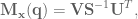
What’s going on here? Here’s what. The Jacobian has dropped rank and become singular (i.e. non-invertible), and when we try to calculate our mass matrix for operational space
the values explode in the inverse calculation. Dropping rank means that the rows of the Jacobian are no longer linearly independent, which means that the matrix can be rotated such that it gives a matrix with a row of zeros. This row of zeros is the degenerate direction, and the problems come from trying to send forces in that direction.
To determine when the Jacobian becomes singular its determinant can be examined; if the determinant of the matrix is zero, then it is singular. Looking the Jacobian for the end-effector:
When it can be that , so the Jacobian becomes
which gives a determinant of
Similarly, when , where and , the Jacobian is
Calculating the determinant of this we get
Note that while in these cases the Jacobian is a square matrix in the event that it is not a square matrix, the determinant of can be found instead.
Fixing the problem
When a singularity is occurring it can be detected, but now it must be handled such that the controller behaves appropriately. This can be done by identifying the degenerate dimensions and setting the force in those directions to zero.
First the SVD decomposition of is found. To get the inverse of this matrix (i.e. to find ) from the returned and matrices is a matter of inverting the matrix :
where is a diagonal matrix of singular values.
Because is diagonal it is very easy to find its inverse, which is calculated by taking the reciprocal of each of the diagonal elements.
Whenever the system approaches a singularity some of the values of will start to get very small, and when we take the reciprocal of them we start getting huge numbers, which is where the value explosion comes from. Instead of allowing this to happen, a check for approaching the singularity can be implemented, which then sets the singular values entries smaller than the threshold equal to zero, canceling out any forces that would be sent in that direction.
Here’s the code:
Mx_inv = np.dot(JEE, np.dot(np.linalg.inv(Mq), JEE.T))
if abs(np.linalg.det(np.dot(JEE,JEE.T))) > .005**2:
    # if we're not near a singularity
    Mx = np.linalg.inv(Mx_inv)
else:
    # in the case that the robot is entering near singularity
    u,s,v = np.linalg.svd(Mx_inv)
    for i in range(len(s)):
        if s[i] < .005: s[i] = 0
        else: s[i] = 1.0/float(s[i])
    Mx = np.dot(v, np.dot(np.diag(s), u.T))
And here’s an animation of the controlled arm now that we’ve accounted for movement when near singular configurations:
As always, the code for this can be found up on my Github. The default is to run using a two link arm simulator written in Python. To run, simply download everything and run the run_this.py file.
Everything is also included required to run the MapleSim arm simulator. To do this, go into the TwoLinkArm folder, and run python setup.py build_ext -i. This should compile the arm simulation to a shared object library that Python can now access on your system. To use it, edit the run_this.py file to import from TwoLinkArm/arm_python to TwoLinkArm/arm and you should be good to go!
More details on getting the MapleSim arm to run can be found in this post.
 ,
,  and
and  denote
  and
and  . It’s important to remember that
  is denoting a velocity, and not a position, as we work through things or it could take you a lot longer to understand than it otherwise might…
![\left[ \begin{array}{c} \dot{\textbf{x}} \\ \pmb{\omega} \end{array} \right] = \textbf{J}(\textbf{q}) \; \dot{\textbf{q}}](https://s0.wp.com/latex.php?latex=%5Cleft%5B+%5Cbegin%7Barray%7D%7Bc%7D+%5Cdot%7B%5Ctextbf%7Bx%7D%7D+%5C%5C+%5Cpmb%7B%5Comega%7D+%5Cend%7Barray%7D+%5Cright%5D+%3D+%5Ctextbf%7BJ%7D%28%5Ctextbf%7Bq%7D%29+%5C%3B+%5Cdot%7B%5Ctextbf%7Bq%7D%7D&bg=ffffff&fg=555555&s=0&c=20201002)
 position of the hand, the angular velocity dimensions are stripped out of the Jacobian so that it’s a 3 x n_joints matrix rather than a 6 x n_joints matrix. So the orientation of the end-effector is not controlled at all. When we did this, we didn’t need to worry or know anything about the form of the angular velocities.
 and
and  , we want to calculate the rotation quaternion
  that takes us from
 here, we negate either the scalar or vector part of the quaternion, but not both.

 is crossed where the arm ‘goes the long way around’. To account for this, use

 is the rotation matrix for the end-effector, and
  is the vector part of the unit quaternion that can be extracted from the rotation matrix
  .
. ,
, and
and  are the scalar and vector part of the quaternion representation of
 is the rotation matrix representing the desired orientation and
 and
and  are the scalar and vector components of the quaternions representing the end-effector and target orientations, respectively, and
  is defined in (Nakanishi eq 73):
![\left[ \begin{array}{ccc} 0 & -\textbf{x}[2] & \textbf{x}[1] \\ \textbf{x}[2] & 0 & -\textbf{x}[0] \\ -\textbf{x}[1] & \textbf{x}[0] & 0 \end{array} \right]](https://s0.wp.com/latex.php?latex=%5Cleft%5B+%5Cbegin%7Barray%7D%7Bccc%7D+0+%26+-%5Ctextbf%7Bx%7D%5B2%5D+%26+%5Ctextbf%7Bx%7D%5B1%5D+%5C%5C+%5Ctextbf%7Bx%7D%5B2%5D+%26+0+%26+-%5Ctextbf%7Bx%7D%5B0%5D+%5C%5C+-%5Ctextbf%7Bx%7D%5B1%5D+%26+%5Ctextbf%7Bx%7D%5B0%5D+%26+0+%5Cend%7Barray%7D+%5Cright%5D&bg=ffffff&fg=555555&s=0&c=20201002)

 cannot be controlled. 2) The rank of the Jacobian determines how many DOF can be controlled at the same time.
 variables can be controlled, but
  cannot be controlled because their corresponding rows are all zeros. So 3 variables can potentially be controlled, but because the Jacobian is rank 2 only two variables can be controlled at a time. If you try to control more than 2 DOF at a time things are going to go poorly. Here are some animations of trying to control 3 DOF vs 2 DOF in a 2 joint arm:


 and
and  are gain terms,
  is the goal state,
  is the system state,
  is the system velocity, and
  is the forcing function.
 implements the obstacle avoidance dynamics, and is a function of the DMP state and velocity. Now then, the question is what are these dynamics exactly?
 , here’s a picture of it:
 , as in the figure below:

 and
and  in the paper, respectively.
 vector to get the cosine of the angle, and then use
 rotated 90 degrees (the
  denoting outer product here). The way I’ve been thinking about this is basically taking your velocity vector,
  axis, and the bottom row by the difference along the
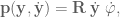
 instead of

 and initial control sequence
 ![\textbf{U} = [u_{t_0}, u_{t_1}, ..., u_{t_{N-1}}]](https://s0.wp.com/latex.php?latex=%5Ctextbf%7BU%7D+%3D+%5Bu_%7Bt_0%7D%2C+u_%7Bt_1%7D%2C+...%2C+u_%7Bt_%7BN-1%7D%7D%5D&bg=ffffff&fg=555555&s=0&c=20201002) .
. to get the trajectory through state space,
  , that results from applying the control sequence
  starting in
  in the state-space and control signal trajectories.
 and evaluate cost of trajectory resulting from
  .
.
 then we've converged and exit.
 , then set
  , and change the update size to be more aggressive. Go back to step 2.
 change the update size to be more modest. Go back to step 3.
 , and dynamics described with the function
 is the input control signal. The trajectory
  is the sequence of states
  that result from applying the control sequence
  starting in the initial state
  .
. , which is the sum of the immediate cost,
  , from each state in the trajectory plus the final cost,
  :
: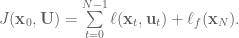
 , we define the cost-to-go as the sum of costs from time
  to
to  :
:
 at time
 that minimizes
  .
.
 and the value function at the next time step:
![V(\textbf{x}) = \min\limits_{\textbf{u}} \left[ \ell(\textbf{x}, \textbf{u}) + V(\textbf{f}(\textbf{x}, \textbf{u})) \right].](https://s0.wp.com/latex.php?latex=V%28%5Ctextbf%7Bx%7D%29+%3D+%5Cmin%5Climits_%7B%5Ctextbf%7Bu%7D%7D+%5Cleft%5B+%5Cell%28%5Ctextbf%7Bx%7D%2C+%5Ctextbf%7Bu%7D%29+%2B+V%28%5Ctextbf%7Bf%7D%28%5Ctextbf%7Bx%7D%2C+%5Ctextbf%7Bu%7D%29%29+%5Cright%5D.&bg=ffffff&fg=555555&s=0&c=20201002)
 to denote the value function at the next time step, which is redundant since
  , but it comes in handy later when they drop the dependencies to simplify notation. So, heads up:
  .
. from which we can calculate the overall cost of the trajectory, and find out the path that the arm will take. To improve things though we’ll need a lot of information about the partial derivatives of the system, calculating these is the second part of the forward rollout phase.
 . For each
  we’ll calculate the derivatives of
  with respect to
  and
and  , which will give us what we need for our linear approximation of the system dynamics.
 and
and  with respect to
  ,
,  ,
,  ,
,  ,
,  ,
,  ,
,  , where the subscripts denote a partial derivative, so
  to be the change in our value function at
  :
:
 is given by:


 , which is the value function at the next time step. NOTE: All of the second derivatives of
  . This control signal update has two parts, a feedforward term,
  , and a feedback term
  . The optimal update is the
  that minimizes the cost of
 and
and 
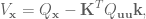

 , and so we’ll simply plug this value in and work backwards in time recursively computing the partial derivatives of
  , for our control signal update. Huzzah! Now all that’s left to do is evaluate this new trajectory. So we set up our system

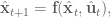
 is less than the cost of
  to get the
  ) stays positive definite, which is important
  position of the hand. These read as “during movement, penalize large control signals, and at the final state, have a big penalty on not being at the target.”

 penalizes the distance from the target, and the cost function during movement is strictly to minimize the control signal, i.e.
  .
.


 always generated the best results, so it was just adding computation time. So I left it out of my implementation. If anyone has insights on an implementation that improves results, please let me know!
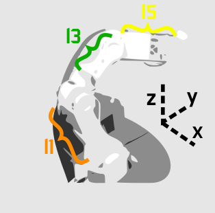
 through
  . The 7th joint,
  , opens and closes the gripper, so we’re safe to ignore it in deriving our Jacobian. The arm segment lengths
  and
and  are named based on the nearest joint angles (makes easier reading in the Jacobian derivation).
 axis, so the rotational part of our transformation matrix
  is
is![^0_\textrm{org}\textbf{R} = \left[ \begin{array}{ccc} \textrm{cos}(q_0) & -\textrm{sin}(q_0) & 0 \\ \textrm{sin}(q_0) & \textrm{cos}(q_0) & 0 \\ 0 & 0 & 1 \end{array} \right],](https://s0.wp.com/latex.php?latex=%5E0_%5Ctextrm%7Borg%7D%5Ctextbf%7BR%7D+%3D+%5Cleft%5B+%5Cbegin%7Barray%7D%7Bccc%7D+%5Ctextrm%7Bcos%7D%28q_0%29+%26+-%5Ctextrm%7Bsin%7D%28q_0%29+%26+0+%5C%5C+%5Ctextrm%7Bsin%7D%28q_0%29+%26+%5Ctextrm%7Bcos%7D%28q_0%29+%26+0+%5C%5C+0+%26+0+%26+1+%5Cend%7Barray%7D+%5Cright%5D%2C&bg=ffffff&fg=555555&s=0&c=20201002)
![^0_\textrm{org}\textbf{D} = \left[ \begin{array}{c} 0 \\ 0 \\ 0 \end{array} \right].](https://s0.wp.com/latex.php?latex=%5E0_%5Ctextrm%7Borg%7D%5Ctextbf%7BD%7D+%3D+%5Cleft%5B+%5Cbegin%7Barray%7D%7Bc%7D+0+%5C%5C+0+%5C%5C+0+%5Cend%7Barray%7D+%5Cright%5D.&bg=ffffff&fg=555555&s=0&c=20201002)
![^0_\textrm{org}\textbf{T} = \left[ \begin{array}{cc} ^0_\textrm{org}\textbf{R} & ^0_\textrm{org}\textbf{D} \\ 0 & 1 \end{array} \right] = \left[ \begin{array}{cccc} \textrm{cos}(q_0) & -\textrm{sin}(q_0) & 0 & 0\\ \textrm{sin}(q_0) & \textrm{cos}(q_0) & 0 & 0 \\ 0 & 0 & 1 & 0 \\ 0 & 0 & 0 & 1 \end{array} \right] .](https://s0.wp.com/latex.php?latex=%5E0_%5Ctextrm%7Borg%7D%5Ctextbf%7BT%7D+%3D+%5Cleft%5B+%5Cbegin%7Barray%7D%7Bcc%7D+%5E0_%5Ctextrm%7Borg%7D%5Ctextbf%7BR%7D+%26+%5E0_%5Ctextrm%7Borg%7D%5Ctextbf%7BD%7D+%5C%5C+0+%26+1+%5Cend%7Barray%7D+%5Cright%5D+%3D+%5Cleft%5B+%5Cbegin%7Barray%7D%7Bcccc%7D+%5Ctextrm%7Bcos%7D%28q_0%29+%26+-%5Ctextrm%7Bsin%7D%28q_0%29+%26+0+%26+0%5C%5C+%5Ctextrm%7Bsin%7D%28q_0%29+%26+%5Ctextrm%7Bcos%7D%28q_0%29+%26+0+%26+0+%5C%5C+0+%26+0+%26+1+%26+0+%5C%5C+0+%26+0+%26+0+%26+1+%5Cend%7Barray%7D+%5Cright%5D+.&bg=ffffff&fg=555555&s=0&c=20201002)
 rotates around the
  . Our transformation matrix looks like
![^1_0\textbf{T} = \left[ \begin{array}{cccc} 1 & 0 & 0 & 0 \\ 0 & \textrm{cos}(q_1) & -\textrm{sin}(q_1) & l_1 \textrm{cos}(q_1) \\ 0 & \textrm{sin}(q_1) & \textrm{cos}(q_1) & l_1 \textrm{sin}(q_1) \\ 0 & 0 & 0 & 1 \end{array} \right] .](https://s0.wp.com/latex.php?latex=%5E1_0%5Ctextbf%7BT%7D+%3D+%5Cleft%5B+%5Cbegin%7Barray%7D%7Bcccc%7D+1+%26+0+%26+0+%26+0+%5C%5C+0+%26+%5Ctextrm%7Bcos%7D%28q_1%29+%26+-%5Ctextrm%7Bsin%7D%28q_1%29+%26+l_1+%5Ctextrm%7Bcos%7D%28q_1%29+%5C%5C+0+%26+%5Ctextrm%7Bsin%7D%28q_1%29+%26+%5Ctextrm%7Bcos%7D%28q_1%29+%26+l_1+%5Ctextrm%7Bsin%7D%28q_1%29+%5C%5C+0+%26+0+%26+0+%26+1+%5Cend%7Barray%7D+%5Cright%5D+.&bg=ffffff&fg=555555&s=0&c=20201002)
 also rotates around the
  . So our transformation matrix looks like
![^2_1\textbf{T} = \left[ \begin{array}{cccc} 1 & 0 & 0 & 0 \\ 0 & \textrm{cos}(q_2) & -\textrm{sin}(q_2) & 0 \\ 0 & \textrm{sin}(q_2) & \textrm{cos}(q_2) & 0 \\ 0 & 0 & 0 & 1 \end{array} \right] .](https://s0.wp.com/latex.php?latex=%5E2_1%5Ctextbf%7BT%7D+%3D+%5Cleft%5B+%5Cbegin%7Barray%7D%7Bcccc%7D+1+%26+0+%26+0+%26+0+%5C%5C+0+%26+%5Ctextrm%7Bcos%7D%28q_2%29+%26+-%5Ctextrm%7Bsin%7D%28q_2%29+%26+0+%5C%5C+0+%26+%5Ctextrm%7Bsin%7D%28q_2%29+%26+%5Ctextrm%7Bcos%7D%28q_2%29+%26+0+%5C%5C+0+%26+0+%26+0+%26+1+%5Cend%7Barray%7D+%5Cright%5D+.&bg=ffffff&fg=555555&s=0&c=20201002)
 axis. This is determined by where
 ![^3_2\textbf{T} = \left[ \begin{array}{cccc} \textrm{cos}(q_3) & 0 & -\textrm{sin}(q_3) & 0\\ 0 & 1 & 0 & l_3 \\ \textrm{sin}(q_3) & 0 & \textrm{cos}(q_3) & 0\\ 0 & 0 & 0 & 1 \end{array} \right] .](https://s0.wp.com/latex.php?latex=%5E3_2%5Ctextbf%7BT%7D+%3D+%5Cleft%5B+%5Cbegin%7Barray%7D%7Bcccc%7D+%5Ctextrm%7Bcos%7D%28q_3%29+%26+0+%26+-%5Ctextrm%7Bsin%7D%28q_3%29+%26+0%5C%5C+0+%26+1+%26+0+%26+l_3+%5C%5C+%5Ctextrm%7Bsin%7D%28q_3%29+%26+0+%26+%5Ctextrm%7Bcos%7D%28q_3%29+%26+0%5C%5C+0+%26+0+%26+0+%26+1+%5Cend%7Barray%7D+%5Cright%5D+.&bg=ffffff&fg=555555&s=0&c=20201002)
 to
to ![^4_3\textbf{T} = \left[ \begin{array}{cccc} 1 & 0 & 0 & 0 \\ 0 & \textrm{cos}(q_4) & -\textrm{sin}(q_4) & 0 \\ 0 & \textrm{sin}(q_4) & \textrm{cos}(q_4) & 0 \\ 0 & 0 & 0 & 1 \end{array} \right] .](https://s0.wp.com/latex.php?latex=%5E4_3%5Ctextbf%7BT%7D+%3D+%5Cleft%5B+%5Cbegin%7Barray%7D%7Bcccc%7D+1+%26+0+%26+0+%26+0+%5C%5C+0+%26+%5Ctextrm%7Bcos%7D%28q_4%29+%26+-%5Ctextrm%7Bsin%7D%28q_4%29+%26+0+%5C%5C+0+%26+%5Ctextrm%7Bsin%7D%28q_4%29+%26+%5Ctextrm%7Bcos%7D%28q_4%29+%26+0+%5C%5C+0+%26+0+%26+0+%26+1+%5Cend%7Barray%7D+%5Cright%5D+.&bg=ffffff&fg=555555&s=0&c=20201002)
![^5_4\textbf{T} = \left[ \begin{array}{cccc} \textrm{cos}(q_5) & 0 & -\textrm{sin}(q_5) & 0 \\ 0 & 1 & 0 & l_5 \\ \textrm{sin}(q_5) & 0 & \textrm{cos}(q_5) & 0\\ 0 & 0 & 0 & 1 \end{array} \right] .](https://s0.wp.com/latex.php?latex=%5E5_4%5Ctextbf%7BT%7D+%3D+%5Cleft%5B+%5Cbegin%7Barray%7D%7Bcccc%7D+%5Ctextrm%7Bcos%7D%28q_5%29+%26+0+%26+-%5Ctextrm%7Bsin%7D%28q_5%29+%26+0+%5C%5C+0+%26+1+%26+0+%26+l_5+%5C%5C+%5Ctextrm%7Bsin%7D%28q_5%29+%26+0+%26+%5Ctextrm%7Bcos%7D%28q_5%29+%26+0%5C%5C+0+%26+0+%26+0+%26+1+%5Cend%7Barray%7D+%5Cright%5D+.&bg=ffffff&fg=555555&s=0&c=20201002)

 . This could be a big ol’ headache to do it by hand, OR we could use SymPy, the symbolic computation package for Python. Which is exactly what we’ll do. So after a quick
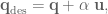
 position of the end-effector, calculate the difference between it and the target end-effector position, use that to generate the end-effector control signal
  , get the Jacobian for the current state of the arm using the function above, find the set of joint torques to apply, approximate this control by generating a set of target joint angles to move to, and then repeat this whole loop until we’re within some threshold of the target position. Whew.
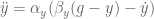 ,
, is the goal, and
  .
. such that you get the desire behaviour is a non-trivial question. The crux of the DMP framework is an additional nonlinear system used to define the forcing function
  .
.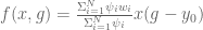 ,
, is the initial position of the system,
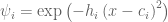 ,
, is a weighting for a given basis function
  . You may recognize that the
  , where
  is the variance. So our forcing function is a set of Gaussians that are ‘activated’ as the canonical system
  term, which is both a ‘diminishing’ and spatial scaling term.
 , and goes to 0 as time goes to infinity. For right now, let’s pretend that
  . The first main point is that there are some basis functions which are activated as a function of
 term of the forcing function handles, by scaling the activation of each of these basis functions to be relative to the distance to the target, causing the system to cover more or less distance. For example, let’s say that we have a set of discrete DMPs set up to follow a given trajectory:


 is equal to the number of basis functions divided by the center of that basis function. When we do this, we can now generate centers for our basis functions that are well spaced out:
 , our temporal scaling term. Given that our system dynamics are:
 ,
, ,
, ,
, (where bold denotes a vector, in this case the time series of desired points in the trajectory), and differentiate it twice to get the accelerations:
 .
. .
. . In locally weighted regression sets up to minimize:
 ,
,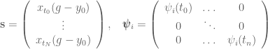
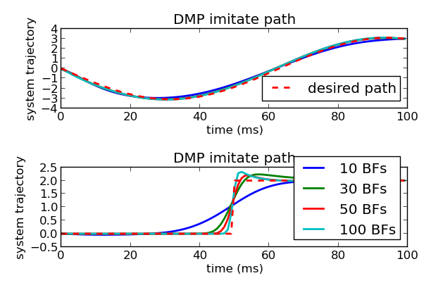


![\textbf{J}(\textbf{q}) = \left[ \begin{array}{cc} -L_0 sin(q_0) - L_1 sin(q_0 + q_1) & -L_1 sin(q_0 + q_1) \\ L_0 cos(q_0) + L_1 cos(q_0 + q_1) & L_1 cos(q_0 + q_1) \end{array} \right].](https://s0.wp.com/latex.php?latex=%5Ctextbf%7BJ%7D%28%5Ctextbf%7Bq%7D%29+%3D+%5Cleft%5B+%5Cbegin%7Barray%7D%7Bcc%7D+-L_0+sin%28q_0%29+-+L_1+sin%28q_0+%2B+q_1%29+%26+-L_1+sin%28q_0+%2B+q_1%29+%5C%5C+L_0+cos%28q_0%29+%2B+L_1+cos%28q_0+%2B+q_1%29+%26+L_1+cos%28q_0+%2B+q_1%29+%5Cend%7Barray%7D+%5Cright%5D.&bg=ffffff&fg=555555&s=0&c=20201002)
 it can be that
  , so the Jacobian becomes
![\textbf{J}(\textbf{q}) = \left[ \begin{array}{cc} (L_0 + L_1)(-sin(q_0)) & -L_1 sin(q_0) \\ (L_0 + L_1) cos(q_0) & L_1 cos(q_0) \end{array} \right],](https://s0.wp.com/latex.php?latex=%5Ctextbf%7BJ%7D%28%5Ctextbf%7Bq%7D%29+%3D+%5Cleft%5B+%5Cbegin%7Barray%7D%7Bcc%7D+%28L_0+%2B+L_1%29%28-sin%28q_0%29%29+%26+-L_1+sin%28q_0%29+%5C%5C+%28L_0+%2B+L_1%29+cos%28q_0%29+%26+L_1+cos%28q_0%29+%5Cend%7Barray%7D+%5Cright%5D%2C&bg=ffffff&fg=555555&s=0&c=20201002)

 , where
  and
and  , the Jacobian is
![\textbf{J}(\textbf{q}) = \left[ \begin{array}{cc} -(L_0 - L_1) sin(q_0) & L_1 sin(q_0) \\ (L_0 + L_1) cos(q_0) & - L_1 cos(q_0) \end{array} \right].](https://s0.wp.com/latex.php?latex=%5Ctextbf%7BJ%7D%28%5Ctextbf%7Bq%7D%29+%3D+%5Cleft%5B+%5Cbegin%7Barray%7D%7Bcc%7D+-%28L_0+-+L_1%29+sin%28q_0%29+%26+L_1+sin%28q_0%29+%5C%5C+%28L_0+%2B+L_1%29+cos%28q_0%29+%26+-+L_1+cos%28q_0%29+%5Cend%7Barray%7D+%5Cright%5D.&bg=ffffff&fg=555555&s=0&c=20201002)

 can be found instead.
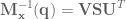 is found. To get the inverse of this matrix (i.e. to find
  ) from the returned
  and
and  :
: