Building models in Mujoco

Mujoco is an awesome simulation tool. You’re probably familiar with it from it’s use in the OpenAI gym, or from it featuring in articles and videos on model predictive control and robots learning to walk research. If you’re not familiar with it, you should check it out! Mujoco provides super fast dynamics simulation with a focus on contact dynamics. It’s especially useful for simulating robotic arms and gripping tasks.

There is a growing model repository, but it’s not unlikely you’re going to want to build your own model. It turns out this is relatively easy in Mujoco. There are two parts to defining a model: 1) The STL files, which are 3D models of the robot components, and 2) the XML file, which specifies the kinematic and dynamic relationships in the model. For STL manipulation, we use the program SketchUp because it is freely available with both offline and online versions.

This post will start by going over some settings in SketchUp assuming you haven’t used it before. We’ll then walk through how to set up the STL files for the individual components of the robot model (assuming that you already have the 3D modeling completed), steps for generating a Mujoco XML robot description file, and go over a couple of the more common problems that come up in the process.

If you don’t have the 3D modeling aleady completed, it’s worth doing a quick search around online to see if someone else has already made it because there are a lot out there not posted officially on any model repo. Github is a good source, and so is https://www.traceparts.com/en. We’re not going to cover any 3D modeling how-to here.

Shout out to my colleague Pawel Jaworski who worked through this process and wrote up the first of this document!

Sketchup Settings – Set model units on import

Before opening your STL, in the open file window select your file and click on the Options button next to Import. Select the units that the model was defined in. If you import your object and cannot see it, it is likely that the units selected during the import were incorrect and the object is simply too small to see.

Skechup Settings – Set model units for export

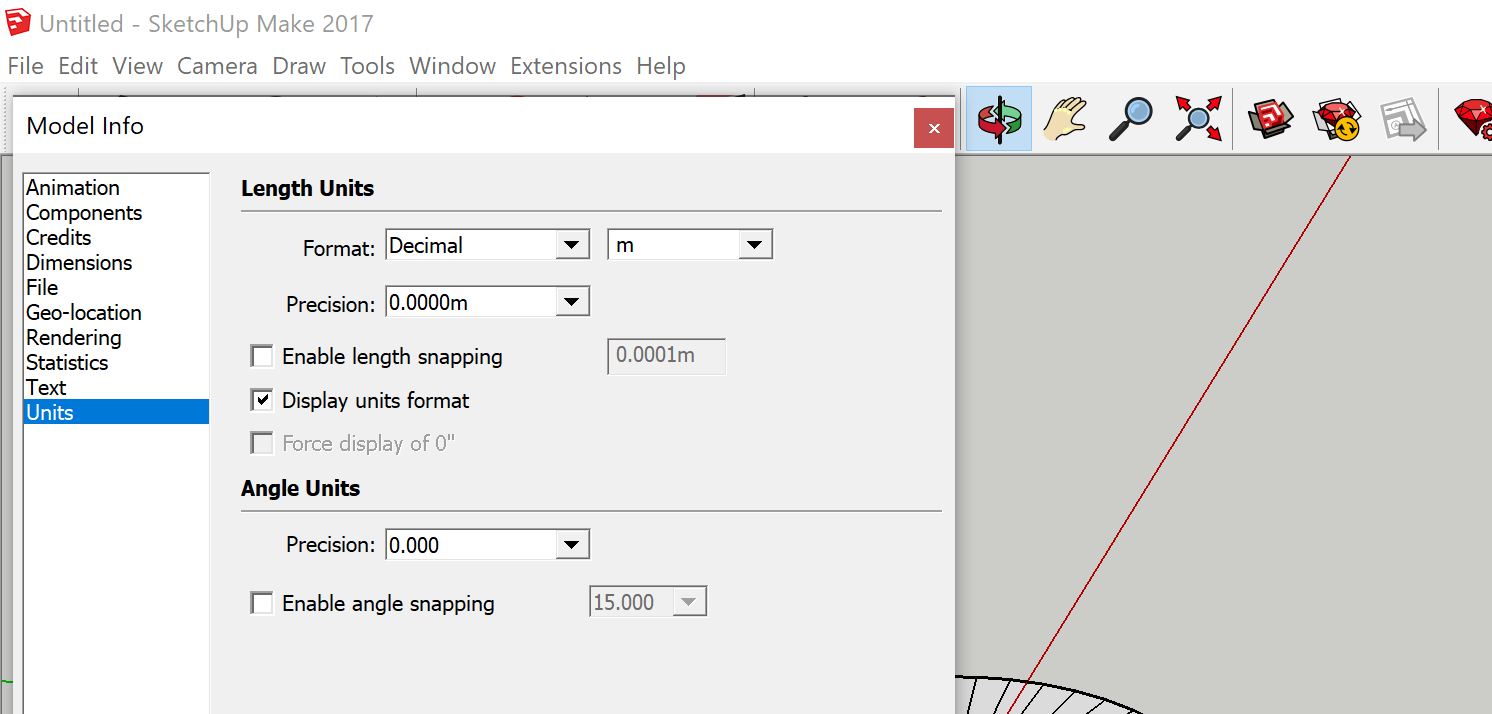
Mujoco uses the units specified in your STL models. ABR Control uses metres, and things generally are easiest when everyone is using the same units. To change your units to meters, go to Model Info > Length Units > 0.0m.

Sketchup Settings – Measurement precision

Before doing any measuring in SketchUp, change your measurement precision in Model Info > Units. precision to the largest number of digits to make sure you get accurate measurements (which you will need when building the Mujoco XML), the default in the online version is 1 significant digit.

Sketchup Settings – Disable snapping

If you are like me then auto-snapping is often a huge pet peeve. To disable it, go to Model Info > Units and unclick Length snapping and Angle snapping.

Sketchup Settings – Xray mode

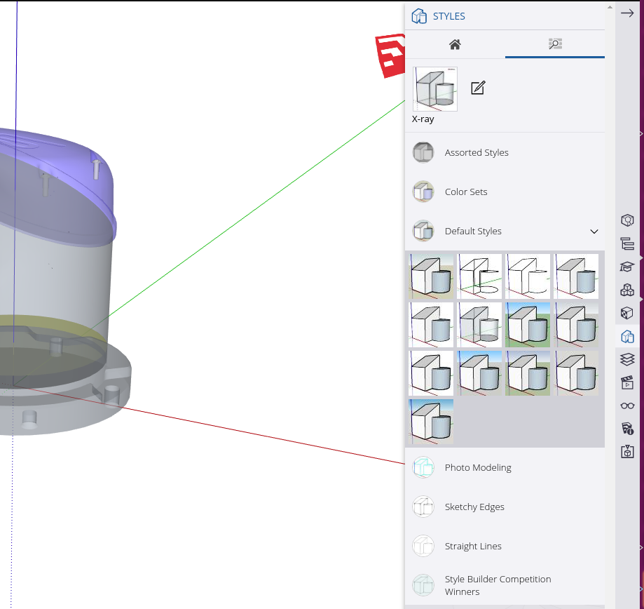
It can be helpful to set the default view to xray mode so you can see inside the model when manipulating the components. To do this go to Styles > Default Styles > X-ray on the right hand side.

---

Generating component STL files

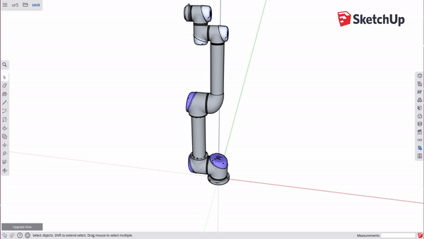
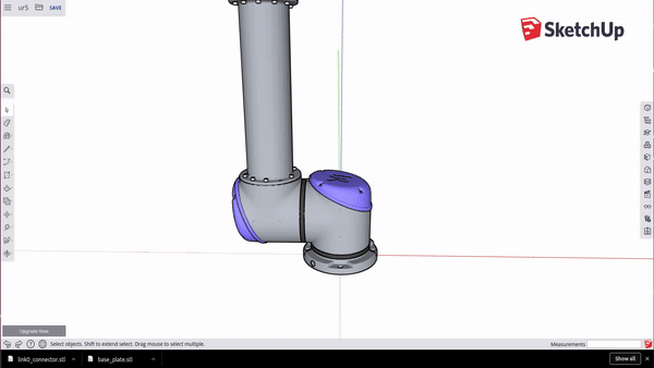
A common starting point for modeling is that you have a 3D model of the full robot. When this is the case, the first step in building a Mujoco model is to generate separate STL files for each of the components of the robot that you want to be able to move independently. For each of these component STL files, we want the point where it connects to the joint to be at the origin (0, 0, 0). We’ve found that this streamlines the process of building the model in the XML and makes it much easier to correctly specify the inertial properties.

If your 3D model is already broken up into each dynamic component (i.e. each arm section that moves independently) then you can skip to the section on centering at the origin.

Exporting components to separate STLs

Make sure you have the model unlocked. To do so, choose the Select tool and highlight the entire model. If the outline is red, it is locked. To unlock it, right click and choose Unlock.

Locked

Unlocked

Unlocking the UR5 model in SketchUp

To get each component piece: Select the entire arm, deselect your component with Ctrl + Shift + Click, and then delete the rest. Go to the folder icon in the top left and select Export > STL. When exporting your model, make sure to not save your model in ASCII format, choose Binary. Repeat this until you have exported every part as its own STL.

How to save an individual component from a complete robot model

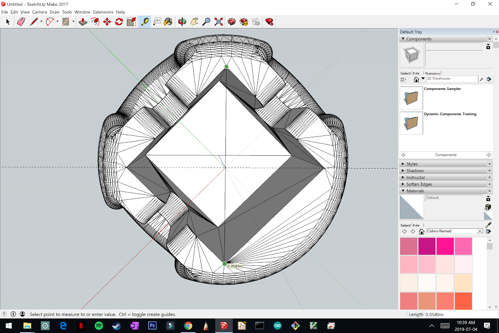
Positioning your object at the origin

For each component, identify where it will connect to the previous component, i.e. where the joint will attach it to the rest of the robot. We want to set up the STL such that this point is at the origin. By doing this we simplify building the XML file later. For the base of the robot this would simply be the bottom of the link, centered.

The easiest way to move the object to the origin is to click a point on the object with the move tool, type [0, 0, 0], and hit enter. This will move the selected point to the origin.

If your object is asymmetrical or you want to center on a point that is difficult to select with your mouse, you can use the measurement tool to set some guidelines. Setting two intersecting lines can help greatly in finding the center of an object (see dotted lines in figure).

Using dotted black guidelines to select an off-center point

Measure the offset distance for the next link

Once the component is appropriately placed at the origin, the next thing we need is the distance to the next attachment point from the origin.

The screenshots below show an example of drawing a verticle guideline to make selecting the next attachment point easy.

Making a verticle reference line that extends beyond the point of interest

Selecting the attachment point of the next component to measure the offset distance

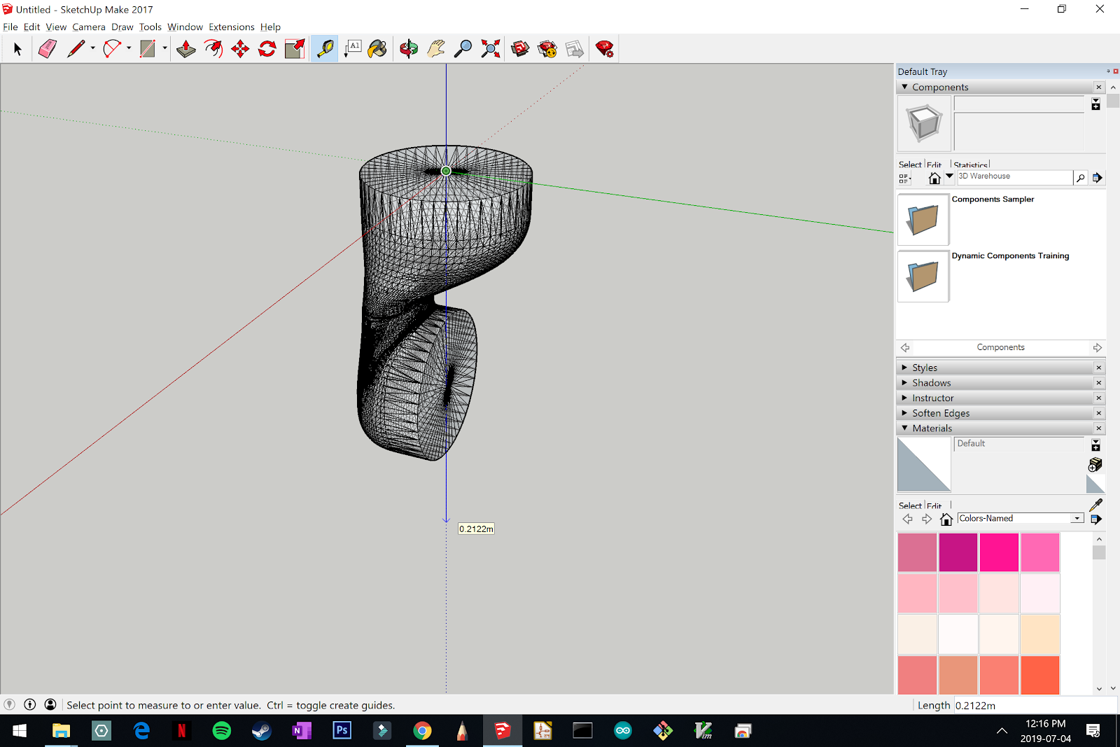
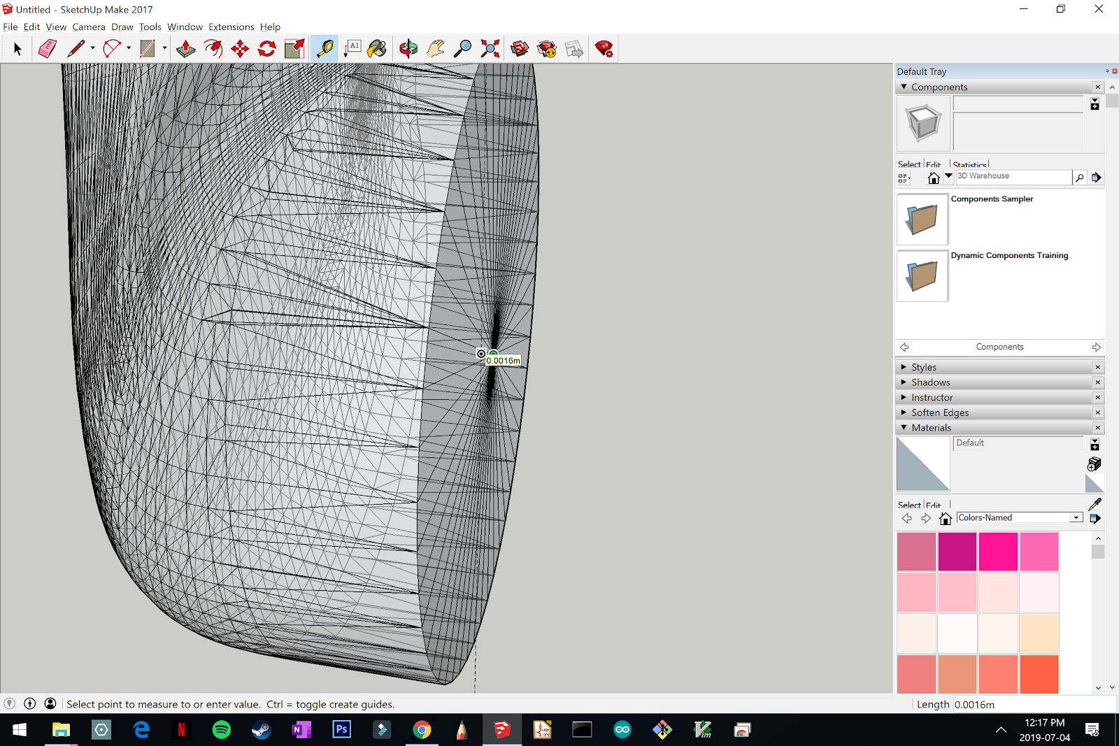
When the next attachment point is selected, the Measurements box will display its coordinates. We will need to know all of the offset distances for each component for building the XML file, so make sure you take note!

Some measuring tips

• Press and hold a directional button while measuring to lock an axis. The up arrow locks the z (blue) axis, the left arrow locks the y (green) axis, and the right arrow locks the x (red) axis.
• The measuring tape line changes color to match an axis colors when it is parallel to any axis.
• Notes on how to use the Tape Measure tool effectively

---

Building your model XML

The easiet way to put together your robot is to build your model up one joint and component at a time, running the simulation to make sure that it works as expected, and then adding the next piece. You will be tempted to assemble a bunch of the model all at once, but this is the siren’s song. You must be strong and resist!

For testing, we created the basic script below, which uses the ABR Control library. To check alignment you can press the space bar to pause the simulation, if you want to make the arm to move then you can change the script to send in some small value instead of zeros.

import mujoco_py as mjp
import glfw
import numpy as np

from abr_control.interfaces.mujoco import Mujoco
from abr_control.arms.mujoco_config import MujocoConfig

robot_config = MujocoConfig(xml_file='example.xml', folder='.')
interface = Mujoco(robot_config, dt=0.001)
interface.connect()

try:
    while True:
        if interface.viewer.exit:
            glfw.destroy_window(interface.viewer.window)
            break

        interface.send_forces(np.zeros(robot_config.N_JOINTS))

finally:
    interface.disconnect()

To run this script with your model, place it in the same directory as your XML file, with a folder called ‘meshes’ that has all of your STLs. If you call your XML file something other than ‘example.xml’ be sure to change that in the script above.

XML model parts

When you’re building your XML file, you’re going to want to have the Mujoco XML Reference constantly open. It’s super detailed and thorough. You can also check out this basic template file on my GitHub which shows the different parts of the file (you will need to fill this out with your own STLs and measurements).

Inside the standard definition tags, the main parts that we’ll be using are:

• <asset> – where you import your STLs using the <mesh> tag
• <worldbody> – where all of the objects in the simulation are defined using <body> tags, including lights, the floor, and of course your robot
• <acutator> – where you specify which joints defined in your robot can be actuated. The ordering of these joints is important, it should be the same as their order in the kinematic tree (i.e. start with joint0 up to the last joint.)

Body building

The meat of the file is of course in the sequence of <body> tags that define the robot model. Each section of the robot looks like this:

<body name="link_n" pos="0 0 0">
    <joint name="joint_n-1" axis="0 0 0" pos="0 0 0"/>
    <geom name="link_n" type="mesh" mesh="shoulder" pos="0 0 0" euler="0 0 0"/>
    <inertial pos="0 0 0" mass="0.01" diaginertia="0 0 0"/>

    <!-- nest the next joint here -->
</body>

Set body position and geoms
Set the offset from the previous body in the pos attribute on the <body> tag, instead of on the geoms. On the <joint> you can then set pos="0 0 0" which we’ve found to help simplify debugging later on.

In each body section you can have several <joint>s and <geom>s. Geoms defined on the same body will be fused together. If you have specific inertia properties for several geoms that are fused together, you will have to create a <body> for each to be able to instantiate their own <inertial> tag. Otherwise, it’s recommended to put them all in the same <body> to optimize simulation speed.

Orientation and inertia
You may need to rotate your STLs to align them properly with the rest of the robot as you build. You can do this either in the <body> or <geom> tags. If you are using an <inertial> tag for this body, we recommend you do this using the euler parameter inside the <geom> tag, instead of inside the <body> tag. If you specify rotation in the <body> tag, you also need to apply the same rotation to your <inertia> parameters, which complicates things.

If you don’t provide an <inertial> tag, the inertia properties will be inferred from the geom.

Contype and conaffinity
If you have geoms that you don’t want to collide with other parts in the model, you can set the contype and conaffinity parameters on the geom tags. This can be handy if you have a tightly-fit 3D model an run into issues with friction, we do this on the UR5 model in the ABR Control library.

End-effector tag for ABR Control
If you’re going to use the ABR Control library operational space controller, you’ll need to add a tag <body name="EE" pos="0 0 0"> at the point of the robot that you want to control. Usually the hand.

Once you’ve added on your robot body segment, save the XML and run the above python script to test out the set up. You will likely need to do some fine tuning by iteratively adjusting the parameters and viewing the model in Mujoco. We’ve found commenting out all of the joints except the joint of interest in the XML file makes assessment much easier.

Template XML file

<mujoco model="example">
    <!-- set some defaults for units and lighting -->
    <compiler angle="radian" meshdir="meshes"/>

    <!-- import our stl files -->
    <asset>
        <mesh file="base.STL" />
        <mesh file="link1.STL" />
        <mesh file="link2.STL" />
    </asset>

    <!-- define our robot model -->
    <worldbody>
        <!-- set up a light pointing down on the robot -->
        <light directional="true" pos="-0.5 0.5 3" dir="0 0 -1" />
        <!-- add a floor so we don't stare off into the abyss -->
        <geom name="floor" pos="0 0 0" size="1 1 1" type="plane" rgba="1 0.83 0.61 0.5"/>
        <!-- the ABR Control Mujoco interface expects a hand mocap -->
        <body name="hand" pos="0 0 0" mocap="true">
            <geom type="box" size=".01 .02 .03" rgba="0 .9 0 .5" contype="2"/>
        </body>

        <!-- start building our model -->
        <body name="base" pos="0 0 0">
            <geom name="link0" type="mesh" mesh="base" pos="0 0 0"/>
            <inertial pos="0 0 0" mass="0" diaginertia="0 0 0"/>

            <!-- nest each child piece inside the parent body tags -->
            <body name="link1" pos="0 0 1">
                <!-- this joint connects link1 to the base -->
                <joint name="joint0" axis="0 0 1" pos="0 0 0"/>

                <geom name="link1" type="mesh" mesh="link1" pos="0 0 0" euler="0 3.14 0"/>
                <inertial pos="0 0 0" mass="0.75" diaginertia="1 1 1"/>

                <body name="link2" pos="0 0 1">
                    <!-- this joint connects link2 to link1 -->
                    <joint name="joint1" axis="0 0 1" pos="0 0 0"/>

                    <geom name="link2" type="mesh" mesh="link2" pos="0 0 0" euler="0 3.14 0"/>
                    <inertial pos="0 0 0" mass="0.75" diaginertia="1 1 1"/>

                    <!-- the ABR Control Mujoco interface uses the EE body to -->
                    <!-- identify the end-effector point to control with OSC-->
                    <body name="EE" pos="0 0.2 0.2">
                        <inertial pos="0 0 0" mass="0" diaginertia="0 0 0" />
                    </body>
                </body>
            </body>
        </body>
    </worldbody>

    <!-- attach actuators to joints -->
    <actuator>
        <motor name="joint0_motor" joint="joint0"/>
        <motor name="joint1_motor" joint="joint1"/>
    </actuator>

</mujoco>

If you want to use the above template XML file with the example Mujoco simulation script withot having to create your own STLs, you can download the meshes folder from ABR Control’s Jaco 2 model to get going. The placement of things is wildly inaccurate but it’ll get you going. You can also checkout the abr_control/arms/jaco2/jaco2.xml and abr_control/arms/ur5/ur5.xml files for more examples.

Hopefully this is enough to get you started, if you run into questions you can post below or on the Mujoco forums. Happy modeling!

---

Troubleshooting

SketchUp – I’m importing my model but I can’t see it

It is likely that the units selected during the import were incorrect and the object is simply too small to see. When opening your STL, in the open file window select your file and click on the options button next to Import to change the units.

Mujoco – My arm isn’t moving, or moves slightly and stops

In this case you likely have collisions between links. You can either add a small gap between links (make sure to account for this shift in subsequent links and joints), or you can use the contype and conaffinity tags to set up the model such that collisions between the two components are not calculated.

For example, in our UR5 model, we set the touching geoms between links to have different contype and conaffinity values so that they don’t scrape against one another and prevent movement.

Mujoco – Parts of my model are spinning around wildly

This usually arises from being instantiated in contact with another part of the model. Sometimes it looks like there is clearly no contact between different model segments, but in fact there is because of how the contact dynamics are calculated.

Only convex shapes are supported. To see the shapes being used to calculate the contact dynamics, press F1 while the model is running. 

• 

  How the STL looks when it’s loaded, lots of space between the neck and jaw

• 

  The actual shapes that are used for calculating contact dynamics.

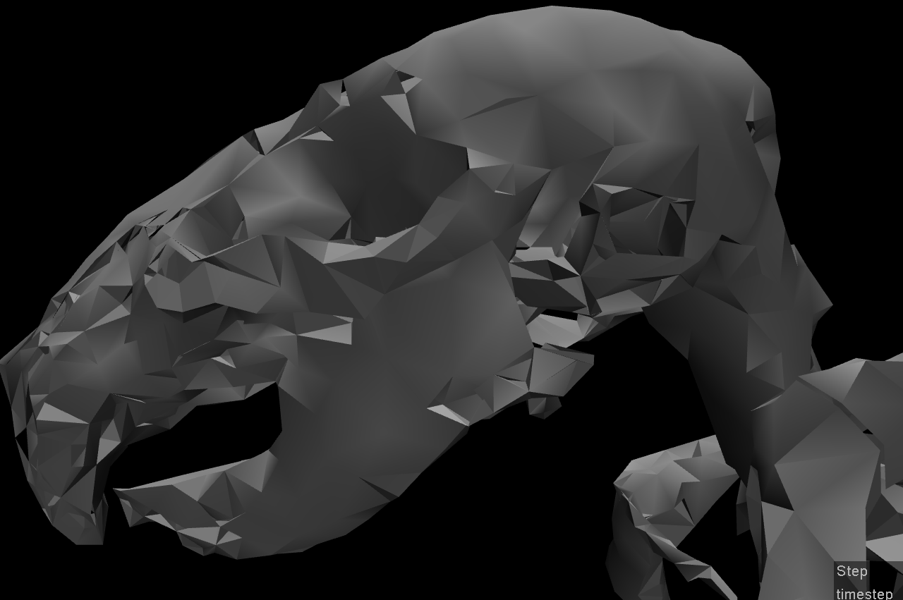
There is no space between the neck and jaw. To address this, you need break things up into multiple component STL files and then stitch them together in the XML. For example, in the above skeleton you would need to break it up into skull and spine STLs. NB: I will not be answering any questions about why a skeleton was used in this example.

Operational space control of 6DOF robot arm with spiking cameras part 2: Deriving the Jacobian

In the previous exciting post in this series I outlined the project, which is in the title, and we worked through getting access to the arm through Python. The next step was deriving the Jacobian, and that’s what we’re going to be talking about in this post!

Alright.
This was a time I was very glad to have a previous post talking about generating transformation matrices, because deriving the Jacobian for a 6DOF arm in 3D space comes off as a little daunting when you’re used to 3DOF in 2D space, and I needed a reminder of the derivation process. The first step here was finding out which motors were what, so I went through and found out how each motor moved with something like the following code:

for ii in range(7):
    target_angles = np.zeros(7, dtype='float32')
    target_angles[ii] = np.pi / 4.0
    rob.move(target_angles)
    time.sleep(1)

and I found that the robot is setup in the figures below

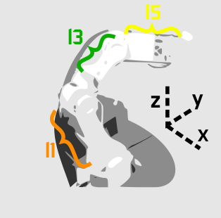
this is me trying my hand at making things clearer using Inkscape, hopefully it’s worked. Displayed are the first 6 joints and their angles of rotation, through . The 7th joint, , opens and closes the gripper, so we’re safe to ignore it in deriving our Jacobian. The arm segment lengths and are named based on the nearest joint angles (makes easier reading in the Jacobian derivation).

Find the transformation matrix from end-effector to origin

So first thing’s first, let’s find the transformation matrices. Our first joint, , rotates around the axis, so the rotational part of our transformation matrix is

and and our origin frame of reference are on top of each other so we don’t need to account for translation, so our translation component of is

Stacking these together to form our first transformation matrix we have

So now we are able to convert a position in 3D space from to the reference frame of joint back to our origin frame of reference. Let’s keep going.

Joint rotates around the axis, and there is a translation along the arm segment . Our transformation matrix looks like

Joint also rotates around the axis, but there is no translation from to . So our transformation matrix looks like

The next transformation matrix is a little tricky, because you might be tempted to say that it’s rotating around the axis, but actually it’s rotating around the axis. This is determined by where is mounted relative to . If it was mounted at 90 degrees from then it would be rotating around the axis, but it’s not. For translation, there’s a translation along the axis up to the next joint, so all in all the transformation matrix looks like:

And then the transformation matrices for coming from to and to are the same as the previous set, so we have

and

Alright! Now that we have all of the transformation matrices, we can put them together to get the transformation from end-effector coordinates to our reference frame coordinates!

At this point I went and tested this with some sample points to make sure that everything seemed to be being transformed properly, but we won’t go through that here.

Calculate the derivative of the transform with respect to each joint

The next step in calculating the Jacobian is getting the derivative of . This could be a big ol’ headache to do it by hand, OR we could use SymPy, the symbolic computation package for Python. Which is exactly what we’ll do. So after a quick

sudo pip install sympy

I wrote up the following script to perform the derivation for us

import sympy as sp

def calc_transform():
    # set up our joint angle symbols (6th angle doesn't affect any kinematics)
    q = [sp.Symbol('q0'), sp.Symbol('q1'), sp.Symbol('q2'), sp.Symbol('q3'),
            sp.Symbol('q4'), sp.Symbol('q5')]
    # set up our arm segment length symbols
    l1 = sp.Symbol('l1')
    l3 = sp.Symbol('l3')
    l5 = sp.Symbol('l5')

    Torg0 = sp.Matrix([[sp.cos(q[0]), -sp.sin(q[0]), 0, 0,],
                       [sp.sin(q[0]), sp.cos(q[0]), 0, 0],
                       [0, 0, 1, 0],
                       [0, 0, 0, 1]])

    T01 = sp.Matrix([[1, 0, 0, 0],
                     [0, sp.cos(q[1]), -sp.sin(q[1]), l1*sp.cos(q[1])],
                     [0, sp.sin(q[1]), sp.cos(q[1]), l1*sp.sin(q[1])],
                     [0, 0, 0, 1]])

    T12 = sp.Matrix([[1, 0, 0, 0],
                     [0, sp.cos(q[2]), -sp.sin(q[2]), 0],
                     [0, sp.sin(q[2]), sp.cos(q[2]), 0],
                     [0, 0, 0, 1]])

    T23 = sp.Matrix([[sp.cos(q[3]), 0, sp.sin(q[3]), 0],
                     [0, 1, 0, l3],
                     [-sp.sin(q[3]), 0, sp.cos(q[3]), 0],
                     [0, 0, 0, 1]])

    T34 = sp.Matrix([[1, 0, 0, 0],
                     [0, sp.cos(q[4]), -sp.sin(q[4]), 0],
                     [0, sp.sin(q[4]), sp.cos(q[4]), 0],
                     [0, 0, 0, 1]])

    T45 = sp.Matrix([[sp.cos(q[5]), 0, sp.sin(q[5]), 0],
                     [0, 1, 0, l5],
                     [-sp.sin(q[5]), 0, sp.cos(q[5]), 0],
                     [0, 0, 0, 1]])

    T = Torg0 * T01 * T12 * T23 * T34 * T45

    # position of the end-effector relative to joint axes 6 (right at the origin)
    x = sp.Matrix([0,0,0,1])

    Tx = T * x

    for ii in range(6):
        print q[ii]
        print sp.simplify(Tx[0].diff(q[ii]))
        print sp.simplify(Tx[1].diff(q[ii]))
        print sp.simplify(Tx[2].diff(q[ii]))

And then consolidated the output using some variable shorthand to write a function that accepts in joint angles and generates the Jacobian:

def calc_jacobian(q):
    J = np.zeros((3, 7))

    c0 = np.cos(q[0])
    s0 = np.sin(q[0])
    c1 = np.cos(q[1])
    s1 = np.sin(q[1])
    c3 = np.cos(q[3])
    s3 = np.sin(q[3])
    c4 = np.cos(q[4])
    s4 = np.sin(q[4])

    c12 = np.cos(q[1] + q[2])
    s12 = np.sin(q[1] + q[2])

    l1 = self.l1
    l3 = self.l3
    l5 = self.l5

    J[0,0] = -l1*c0*c1 - l3*c0*c12 - l5*((s0*s3 - s12*c0*c3)*s4 + c0*c4*c12)
    J[1,0] = -l1*s0*c1 - l3*s0*c12 + l5*((s0*s12*c3 + s3*c0)*s4 - s0*c4*c12)
    J[2,0] = 0

    J[0,1] = (l1*s1 + l3*s12 + l5*(s4*c3*c12 + s12*c4))*s0
    J[1,1] = -(l1*s1 + l3*s12 + l5*s4*c3*c12 + l5*s12*c4)*c0
    J[2,1] = l1*c1 + l3*c12 - l5*(s4*s12*c3 - c4*c12)

    J[0,2] = (l3*s12 + l5*(s4*c3*c12 + s12*c4))*s0
    J[1,2] = -(l3*s12 + l5*s4*c3*c12 + l5*s12*c4)*c0
    J[2,2] = l3*c12 - l5*(s4*s12*c3 - c4*c12)

    J[0,3] = -l5*(s0*s3*s12 - c0*c3)*s4
    J[1,3] = l5*(s0*c3 + s3*s12*c0)*s4
    J[2,3] = -l5*s3*s4*c12

    J[0,4] = l5*((s0*s12*c3 + s3*c0)*c4 + s0*s4*c12)
    J[1,4] = l5*((s0*s3 - s12*c0*c3)*c4 - s4*c0*c12)
    J[2,4] = -l5*(s4*s12 - c3*c4*c12)

    return J

Alright! Now we have our Jacobian! Really the only time consuming part here was calculating our end-effector to origin transformation matrix, generating the Jacobian was super easy using SymPy once we had that.

Hack position control using the Jacobian

Great! So now that we have our Jacobian we’ll be able to translate forces that we want to apply to the end-effector into joint torques that we want to apply to the arm motors. Since we can’t control applied force to the motors though, and have to pass in desired angle positions, we’re going to do a hack approximation. Let’s first transform our forces from end-effector space into a set of joint angle torques:

To approximate the control then we’re simply going to take the current set of joint angles (which we know because it’s whatever angles we last told the system to move to) and add a scaled down version of to approximate applying torque that affects acceleration and then velocity.

where is the gain term, I used .001 here because it was nice and slow, so no crazy commands that could break the servos would be sent out before I could react and hit the cancel button.

What we want to do then to implement operational space control here then is find the current position of the end-effector, calculate the difference between it and the target end-effector position, use that to generate the end-effector control signal , get the Jacobian for the current state of the arm using the function above, find the set of joint torques to apply, approximate this control by generating a set of target joint angles to move to, and then repeat this whole loop until we’re within some threshold of the target position. Whew.

So, a lot of steps, but pretty straight forward to implement. The method I wrote to do it looks something like:

def move_to_xyz(self, xyz_d):
    """
    np.array xyz_d: 3D target (x_d, y_d, z_d)
    """
    count = 0
    while (1):
        count += 1
        # get control signal in 3D space
        xyz = self.calc_xyz()
        delta_xyz = xyz_d - xyz
        ux = self.kp * delta_xyz

        # transform to joint space
        J = self.calc_jacobian()
        u = np.dot(J.T, ux)

        # target joint angles are current + uq (scaled)
        self.q[...] += u * .001
        self.robot.move(np.asarray(self.q.copy(), 'float32'))

        if np.sqrt(np.sum(delta_xyz**2)) < .1 or count > 1e4:
            break

And that is it! We have successfully hacked together a system that can perform operational space control of a 6DOF robot arm. Here is a very choppy video of it moving around to some target points in a grid on a cube.

So, granted I had to drop a lot of frames from the video to bring it’s size down to something close to reasonable, but still you can see that it moves to target locations super fast!

Alright this is sweet, but we’re not done yet. We don’t want to have to tell the arm where to move ourselves. Instead we’d like the robot to perform target tracking for some target LED we’re moving around, because that’s way more fun and interactive. To do this, we’re going to use spiking cameras! So stay tuned, we’ll talk about what the hell spiking cameras are and how to use them for a super quick-to-setup and foolproof target tracking system in the next exciting post!

Operational space control of 6DOF robot arm with spiking cameras part 1: Getting access to the arm through Python

From June 9th to the 19th we ran a summer school (brain camp) in our lab with people from all over to come and learn how to use our neural modeling software, Nengo, and then work on a project with others in the school and people from the lab. We had a bunch of fun hardware available, from neuromorphic hardware from the SpiNNaker group over at Cambridge to lego robots on omni-wheels to spiking cameras (i’ll discuss what a spiking camera is exactly in part 3 of this series) and little robot arms. There were a bunch of awesome projects, people built neural models capable of performing a simplified version of the Wisconsin card sorting task that they then got running on the SpiNNaker boards, a neural controller built to move a robot leech, a spiking neurons reinforcement-learning system implemented on SpiNNaker with spiking cameras to control the lego robot that learned to move towards green LEDs and avoid red LEDs, and a bunch of others. If you’re interested in participating in these kinds of projects and learning more about this I highly suggest you apply to the summer school for next year!

I took the summer school as a chance to break from other projects and hack together a project. The idea was to take the robot arm, implement an operational space controller (i.e. find the Jacobian), and then used spiking cameras to track an LED and have the robot arm learn how to move to the target, no matter where the cameras were placed, by learning the relationship between where the target is in camera-centric coordinates and arm-centric coordinates. This broke down into several steps: 1) Get access to the arm through Python, 2) derive the Jacobian to implement operational space control, 3) sample state space to get an approximation of the camera-centric to arm-centric function, 4) implement the control system to track the target LED.

Here’s a picture of the set-up during step 3, training.

So in the center is the 6DOF robot arm with a little LED attached to the head, and highlighted in orange circles are the two spiking cameras, expertly taped to the wall with office-grade scotch tape. You can also see the SpiNNaker board in the top left as a bonus, but I didn’t have enough time to involve it in this project.

I was originally going to write this all up as one post, because the first two parts are re-implementing previous posts, but even skimming through those steps it was getting long and I’m sure no one minds having a few different examples to look through for generating Cython code or deriving a Jacobian. So I’m going to break this into a few parts. Here in this post we’ll work through the first step (Cython) of our journey.

Get access to the arm through Python

The arm we had was the VE026A Denso training robot, on loan from Dr. Bryan Tripp of the neuromorphic robotics lab at UW. Previously an interface had been built up by one of Dr. Tripp’s summer students, written in C. C is great and all but Python is much easier to work with, and the rest of the software I wanted to work you know what I’m done justifying it Python is just great so Python is what I wanted to use. The end.

So to get access to the arm in Python I used the great ol’ C++ wrapper hack described in a previous post. Looking at Murphy-the-summer-student’s C code there were basically three functions I needed access to:

// initialize threads, connect to robot
void start_robot(int *semid, int32_t *ctrlid, int32_t *robotid, float **angles)
// send a set of joint angles to the robot servos
void Robot_Execute_slvMove(int32_t robotid, float j1, float j2, float j3, float j4, float j5, float j6, float j7, float j8)
// kill threads, disconnect from robot
void stop_robot(int semid, int32_t ctrlid, int32_t robotid)

So I changed the extension of the file to ‘.cpp’ (I know, I know, I said this was a hack!), fixed some compiler errors that popped up, and then appended the following to the end of the file:

/* A class to contain all the information that needs to
be passed around between these functions, and can
encapsulate it and hide it from the Python interface.

Written by Travis DeWolf (June, 2015)
*/

class Robot {
/* Very simple class, just stores the variables
* needed for talking to the robot, and a gives access
* to the functions for moving it around */

int semid;
int32_t ctrlid;
int32_t robotid;
float* angles;

public:
Robot();
~Robot();
void connect();
void move(float* angles_d);
void disconnect();
};

Robot::Robot() { }

Robot::~Robot() { free(angles); }

/* Connect to the robot, get the ids and current joint angles */
/* char* usb_port: the name of the port the robot is connected to */
void Robot::connect()
{
start_robot(&semid, &ctrlid, &robotid, &angles);
printf("%i %i %i", robotid, ctrlid, semid);
}

/* Move the robot to the specified angles */
/* float* angles: the target joint angles */
void Robot::move(float* angles)
{
// convert from radians to degrees
Robot_Execute_slvMove(robotid,
angles[0] * 180.0 / 3.14,
angles[1] * 180.0 / 3.14,
angles[2] * 180.0 / 3.14,
angles[3] * 180.0 / 3.14,
angles[4] * 180.0 / 3.14,
angles[5] * 180.0 / 3.14,
angles[6] * 180.0 / 3.14,
angles[7] * 180.0 / 3.14);
}

/* Disconnect from the robot */
void Robot::disconnect()
{
stop_robot(semid, ctrlid, robotid);
}

int main()
{
Robot robot = Robot();
// connect to robot
robot.connect();

// move robot to some random target angles
float target_angles[7] = {0, np.pi / 2.0, 0.0, 0, 0, 0, 0};
robot.move(target_angles);

sleep(1);

// disconnect
robot.disconnect();

return 0;
}

So very simple class. Basically just wanted to create a set of functions to hide some of the unnecessary parameters from Python, do the conversion from radians to degrees (who works in degrees? honestly), and have a short little main function to test the creation of the class, and connection, movement, and disconnection of the robot. Like I said, there were a few compiler errors when switching from C to C++, but really that was the only thing that took any time on this part. A few casts and everything was gravy.

The next part was writing the Cython pyRobot.pyx file (I describe the steps involved in this in more detail in this post):

import numpy as np
cimport numpy as np

cdef extern from "bcap.cpp":
cdef cppclass Robot:
Robot()
void connect()
void move(float* angles)
void disconnect()

cdef class pyRobot:
cdef Robot* thisptr

def __cinit__(self):
self.thisptr = new Robot()

def __dealloc__(self):
del self.thisptr

def connect(self):
"""
Set up the connection to the robot, pass in a vector,
get back the current joint angles of the arm.
param np.ndarray angles: a vector to store current joint angles
"""
self.thisptr.connect()

def move(self, np.ndarray[float, mode="c"] angles):
"""
Step the simulation forward one timestep. Pass in target angles,
get back the current arm joint angles.
param np.ndarray angles: 7D target angle vector
"""
self.thisptr.move(&angles[0])

def disconnect(self):
"""
Disconnect from the robot.
"""
self.thisptr.disconnect()

the setup.py file:

from distutils.core import setup
from distutils.extension import Extension
from Cython.Distutils import build_ext

setup(
name = 'Demos',
ext_modules=[
Extension("test",
sources=["pyRobot.pyx"],
language="c++"),
],
cmdclass = {'build_ext': build_ext},

)

and then compiling!

run setup.py build_ext -i

With all of this working, a nice test.so file was created, and it was now possible to connect to the robot in Python with

import test
rob = test.pyRobot()
rob.connect()
target_angles = np.array([0, np.pi/2, 0, np.pi/4, 0, 0, 0, 0], dtype='float32')
rob.move(target_angles)
import time
time.sleep(1)
rob.disconnect()

In the above code we’re instantiating the pyRobot class, connecting to the robot, defining a set of target angles and telling the robot to move there, waiting for 1 second to give the robot time to actually move, and then disconnecting from the robot. Upon connection we have to pass in a set of joint angles for the servos, and so you see the robot arm jerk into position, and then move to the target set of joint angles, it looks something exactly like this:

Neat, phase 1 complete.

At the end of phase 1 we are able to connect to the robot arm through Python and send commands in terms of joint angles. But we don’t want to send commands in terms of joint angles, we want to just specify the end-effector position and have the robot work out the angles! I’ve implemented an inverse kinematics solver using constrained optimization before for a 3-link planar arm, but we’re not going to go that route. Find out what we’ll do by joining us next time! or by remembering what I said we’d do at the beginning of this post.