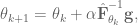
Natural policy gradient in TensorFlow

In working towards reproducing some results from deep learning control papers, one of the learning algorithms that came up was natural policy gradient. The basic idea of natural policy gradient is to use the curvature information of the of the policy’s distribution over actions in the weight update. There are good resources that go into details about the natural policy gradient method (such as here and here), so I’m not going to go into details in this post. Rather, possibly just because I’m new to TensorFlow, I found implementing this method less than straightforward due to a number of unexpected gotchyas. So I’m going to quickly review the algorithm and then mostly focus on the implementation issues that I ran into.

If you’re not familiar with policy gradient or various approaches to the cart-pole problem I also suggest that you check out this blog post from KV Frans, which provides the basis for the code I use here. All of the code that I use in this post is available up on my GitHub, and it’s worth noting this code is for TensorFlow 1.7.0.

Natural policy gradient review

Let’s informally define our notation

$s_t$ and $a_t$ are the system state and chosen action at time $t$
$\theta$ are the network parameters that we’re learning
$\pi_\theta$ is the control policy network parameterized $\theta$
$A^\pi(s_t, a_t, t)$ is the advantage function, which returns the estimated total reward for taking action $a_t$ in state $s_t$ relative to default behaviour (i.e. was this action better or worse than what we normally do)

The regular policy gradient is calculated as:

$\textbf{g} = \frac{1}{T}\sum_{t=0}^T \nabla_\theta \; \textrm{log} \; \pi_\theta(a_t | s_t) \; \hat{A}^\pi(s_t, a_t, t),$

where $\nabla_\theta$ denotes calculating the partial derivative with respect to $\theta$ , the hat above $A^\pi$ denotes that we’re using an estimation of the advantage function, and $\pi_\theta(a_t | s_t)$ returns a scalar value which is the probability of the chosen action $a_t$ in state $s_t$ .

For the natural policy gradient, we’re going to calculate the Fisher information matrix, $F$ , which estimates the curvature of the control policy:

$\hat{F}_{\theta_k} = \frac{1}{T} \sum_{t=0}^T \nabla_\theta \; \textrm{log} \; \pi_\theta(a_t | s_t) \; \nabla_\theta \; \textrm{log} \; \pi_\theta (a_t | s_t)^T.$

The goal of including curvature information is to be able move along the steepest ascent direction, which we estimate with $\hat{\textbf{F}}^{-1}_{\theta_k}$ . Including this then the weight update becomes

$\theta_{k+1} = \theta_k + \alpha \hat{\textbf{F}}^{-1}_{\theta_k} \textbf{g},$

where $\alpha$ is a learning rate parameter. In his paper Towards Generalization and Simplicity in Continuous Control, Aravind Rajeswaran notes that empirically it’s difficult to choose an appropriate $\alpha$ value or set an appropriate schedule. To address this, they normalize the update under the Fisher metric:

$\theta_{k+1} = \theta_k + \sqrt{\frac{\delta}{\textbf{g}^T\hat{\textbf{F}}^{-1}_{\theta_k}\textbf{f}}} \; \hat{\textbf{F}}^{-1}_{\theta_k} \textbf{g}.$

Using the above for the learning rate can be thought of as choosing a step size $\delta$ that is normalized with respect to the change in the control policy. This is beneficial because it means that we don’t do any parameter updates that will drastically change the output of the policy network.

Here’s what the pseudocode for the algorithm looks like

Initialize policy parameters $\theta_0$
for k = 1 to K do:
- collect N trajectories by rolling out the stochastic policy $\pi_{\theta_k}$
- compute $\nabla_\theta \; \textrm{log} \; \pi_\theta(a_t | s_t)$ for each $(s, a)$ pair along the trajectories sampled
- compute advantages $\hat{A}^\pi_k$ based on the sampled trajectories and the estimated value function $V^\pi_{k-1}$
- compute the policy gradient $g$ as specified above
- compute the Fisher matrix and perform the weight update as specified above
- update the value network to get $V^\pi_k$

OK great! On to implementation.

Implementation in TensorFlow 1.7.0

Calculating the gradient at every time step

In TensorFlow, the tf.gradient(ys, xs) function, which calculates the partial derivative of ys with respect to xs:

$\nabla_{X} Y$

will automatically sum over over all elements in ys. There is no function for getting the gradient of each individual entry (i.e. the Jacobian) in ys, which is less than great. People have complained, but until some update happens we can address this with basic list comprehension to iterate through each entry in the history and calculate the gradient at that point in time. If you have a faster means that you’ve tested please comment below!

The code for this looks like

        g_log_prob = tf.stack(
            [tf.gradients(action_log_prob_flat[i], my_variables)[0]
                for i in range(action_log_prob_flat.get_shape()[0])])

Where the result is called g_log_prob_flat because it’s the gradient of the log probability of the chosen action at each time step.

Inverse of a positive definite matrix with rounding errors

One of the problems I ran into was in calculating the normalized learning rate $\sqrt{\frac{\delta}{\textbf{g}^T\hat{\textbf{F}}^{-1}_{\theta_k}\textbf{f}}}$ was that the square root calculation was dying because negative values were being set in. This was very confusing because $\hat{\textbf{F}}$ is a positive definite matrix, which means that $\hat{\textbf{F}}^{-1}$ is also positive definite, which means that $\textbf{x}^T \hat{\textbf{F}}^{-1} \textbf{x} \geq 0$ for any $\textbf{x}$ .

So it was clear that it was a calculation error somewhere, but I couldn’t find the source of the error for a while, until I started doing the inverse calculation myself using SVD to explicitly look at the eigenvalues and make sure they were all > 0. Turns out that there were some very, very small eigenvalues with a negative sign, like -1e-7 kind of range. My guess (and hope) is that these are just rounding errors, but they’re enough to mess up the calculations of the normalized learning rate. So, to handle this I explicitly set those values to zero, and that took care of that.

        S, U, V = tf.svd(F)
        atol = tf.reduce_max(S) * 1e-6
        S_inv = tf.divide(1.0, S)
        S_inv = tf.where(S < atol, tf.zeros_like(S), S_inv)
        S_inv = tf.diag(S_inv)
        F_inv = tf.matmul(S_inv, tf.transpose(U))
        F_inv = tf.matmul(V, F_inv)

Manually adding an update to the learning parameters

Once the parameter update is explicitly calculated, we then need to update them. To implement an explicit parameter update in TensorFlow we do

        # update trainable parameters
        my_variables[0] = tf.assign_add(my_variables[0], update)

So to update the parameters then we call sess.run(my_variables, feed_dict={...}). It’s worth noting here too that any time you run the session with my_variables the parameter update will be calculated and applied, so you can’t run the session with my_variables to only fetch the current values.

Results on the CartPole problem

Now running the original policy gradient algorithm against the natural policy gradient algorithm (with everything else the same) we can examine the results of using the Fisher information matrix in the update provides some strong benefits. The plot below shows the maximum reward received in a batch of 200 time steps, where the system receives a reward of 1 for every time step that the pole stays upright, and 200 is the maximum reward achievable.
Natural_policy_gradient
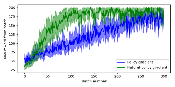
To generate this plot I ran 10 sessions of 300 batches, where each batch runs as many episodes as it takes to get 200 time steps of data. The solid lines are the mean value at each epoch across all sessions, and the shaded areas are the 95% confidence intervals. So we can see that the natural policy gradient starts to hit a reward of 200 inside 100 batches, and that the mean stays higher than normal policy gradient even after 300 batches.

It’s also worth noting that for both the policy gradient and natural policy gradient the average time to run a batch and weight update was about the same on my machine, between 150-180 milliseconds.

The modified code for policy gradient, the natural policy gradient, and plotting code are all up on my GitHub.

Other notes

Had to reduce the $\delta$ to 0.001 (from 0.05 which was used in the Rajeswaran paper) to get the learning to converge, suspect this is because of the greatly reduced complexity of the space and control problem.
The Rajeswaran paper algorithm does gradient ascent instead of descent, which is why the signs are how they are.

studywolf

a blog for things I encounter while coding and researching neuroscience, motor control, and learning