Robot control part 3: Accounting for mass and gravity

In the exciting previous post we looked at how to go about generating a Jacobian matrix, which we could use to transformation both from joint angle velocities to end-effector velocities, and from desired end-effector forces into joint angle torques. I briefly mentioned right at the end that using just this force transformation to build your control signal was only appropriate for very simple systems that didn’t have to account for things like arm-link mass or gravity.

In general, however, mass and gravity must be accounted for and cancelled out. The full dynamics of a robot arm are

$\textbf{M}(\textbf{q}) \ddot{\textbf{q}} = (\textbf{u} - \textbf{C}(\textbf{q}, \dot{\textbf{q}}) - \textbf{g}(\textbf{q})) ,$

where $\ddot{\textbf{q}}$ is joint angle acceleration, $\textbf{u}$ is the control signal (specifying torque), $\textbf{C}(\textbf{q}, \dot{\textbf{q}})$ is a function describing the Coriolis and centrifugal effects, $\textbf{g}(\textbf{q})$ is the effect of gravity in joint space, and $\textbf{M}$ is the mass matrix of the system in joint space.

There are a lot of terms involved in the system acceleration, so while the Jacobian can be used to transform forces between coordinate systems it is clear that just setting the control signal $\textbf{u} = \textbf{J}_{ee}^T (\textbf{q})\textbf{F}_\textbf{x}$ is not sufficient, because a lot of the dynamics affecting acceleration aren’t accounted for. In this section an effective PD controller operating in joint space will be developed that will allow for more precise control by cancelling out unwanted acceleration terms. To do this the effects of inertia and gravity need to be calculated.

Accounting for inertia

The fact that systems have mass is a pain in our controller’s side because it introduces inertia into our system, making control of how the system will move at any given point in time more difficult. Mass can be thought of as an object’s unwillingness to respond to applied forces. The heavier something is, the more resistant it is to acceleration, and the force required to move a system along a desired trajectory depends on both the object’s mass and its current acceleration.

To effectively control a system, the system inertia needs to be calculated so that it can be included in the control signal and cancelled out.

Given the robot arm above, operating in the $(x,z)$ plane, with the $y$ axis extending into the picture where the yellow circles represent each links centre-of-mass (COM). The position of each link is COM is defined relative to that link’s reference frame, and the goal is to figure out how much each link’s mass will affect the system dynamics.

The first step is to transform the representation of each of the COM from Cartesian coordinates in the reference frame of their respective arm segments into terms of joint angles, such that the Jacobian for each COM can be calculated.

Let the COM positions relative to each segment’s coordinate frame be

$\textrm{com}_0 = \left[ \begin{array}{c} \frac{1}{2}cos(q_0) \\ 0 \\ \frac{1}{2}sin(q_0) \end{array} \right], \;\;\;\; \textrm{com}_1 = \left[ \begin{array}{c} \frac{1}{4}cos(q_1) \\ 0 \\ \frac{1}{4}sin(q_1) \end{array} \right].$

The first segment’s COM is already in base coordinates (since the first link and the base share the same coordinate frame), so all that is required is the position of the second link’s COM in the base reference frame, which can be done with the transformation matrix

$^1_0\textbf{T} = \left[ \begin{array}{cccc} cos(q_1) & 0 & -sin(q_1) & L_0 cos(q_0) \\ 0 & 1 & 0 & 0 \\ sin(q_1) & 0 & cos(q_1) & L_0 sin(q_0) \\ 0 & 0 & 0 & 1 \end{array} \right].$

Using $^1_0\textbf{T}$ to transform the $\textrm{com}_1$ gives

$^1_0\textbf{T} \; \textrm{com}_1 = \left[ \begin{array}{cccc} cos(q_1) & 0 & -sin(q_1) & L_0 cos(q_0) \\ 0 & 1 & 0 & 0 \\ sin(q_1) & 0 & cos(q_1) & L_0 sin(q_0) \\ 0 & 0 & 0 & 1 \end{array} \right] \; \; \left[ \begin{array}{c} \frac{1}{4}cos(q_1) \\ 0 \\ \frac{1}{4}sin(q_1) \\ 1 \end{array} \right]$

$^1_0\textbf{T} \; \textrm{com}_1 = \left[ \begin{array}{c} L_0 cos(q_0) + \frac{1}{4}cos(q_0 + q_1) \\ 0 \\ L_0 sin(q_0) + \frac{1}{4} cos(q_0 + q_1) \\ 1 \end{array} \right].$

To see the full computation worked out explicitly please see my previous robot control post.

Now that we have the COM positions in terms of joint angles, we can find the Jacobians for each point through our Jacobian equation:

$\textbf{J} = \frac{\partial \textbf{x}}{\partial \textbf{q}}$ .

Using this for each link gives us:

$\textbf{J}_0 = \left[ \begin{array}{cc} -\frac{1}{2}sin(q_0) & 0 \\ 0 & 0 \\ \frac{1}{2} cos(q_0) & 0 \\ 0 & 0 \\ 1 & 0 \\ 0 & 0 \end{array} \right]$
$\textbf{J}_1 = \left[ \begin{array}{cc} -L_0sin(q_0) -\frac{1}{4}sin(\theta_0 + q_1) & -\frac{1}{4} sin(q_0 + \theta_1) \\ 0 & 0 \\ L_0 cos(q_0) + \frac{1}{4}cos(q_0 + q_1) & \frac{1}{4} cos(q_0 +q_1) \\ 0 & 0 \\ 1 & 1 \\ 0 & 0 \end{array} \right]$ .

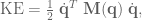
Kinetic energy

The total energy of a system can be calculated as a sum of the energy introduced from each source. The Jacobians just derived will be used to calculate the kinetic energy each link generates during motion. Each link’s kinetic energy will be calculated and summed to get the total energy introduced into the system by the mass and configuration of each link.

Kinetic energy (KE) is one half of mass times velocity squared:

$\textrm{KE} = \frac{1}{2} \; \dot{\textbf{x}}^T \textbf{M}_\textbf{x}(\textbf{q}) \; \dot{\textbf{x}},$

where $\textbf{M}_\textbf{x}$ is the mass matrix of the system, with the subscript $\textbf{x}$ denoting that it is defined in Cartesian space, and $\dot{\textbf{x}}$ is a velocity vector, where $\dot{\textbf{x}}$ is of the form

$\dot{\textbf{x}} = \left[ \begin{array}{c} \dot{x} \\ \dot{y} \\ \dot{z} \\ \dot{\omega_x} \\ \dot{\omega_y} \\ \dot{\omega_z} \end{array} \right],$

and the mass matrix is structured

$\textbf{M}_{\textbf{x}_i} (\textbf{q})= \left[ \begin{array}{cccccc} m_i & 0 & 0 & 0 & 0 & 0 \\ 0 & m_i & 0 & 0 & 0 & 0 \\ 0 & 0 & m_i & 0 & 0 & 0 \\ 0 & 0 & 0 & I_{xx} & I_{xy} & I_{xz} \\ 0 & 0 & 0 & I_{yx} & I_{yy} & I_{yz} \\ 0 & 0 & 0 & I_{zx} & I_{zy} & I_{zz} \end{array} \right],$

where $m_i$ is the mass of COM $i$ , and the $I_{ij}$ terms are the moments of inertia, which define the object’s resistance to change in angular velocity about the axes, the same way that the mass element defines the object’s resistance to changes in linear velocity.

As mentioned above, the mass matrix for the COM of each link is defined in Cartesian coordinates in its respective arm segment’s reference frame. The effects of mass need to be found in joint angle space, however, because that is where the controller operates. Looking at the summation of the KE introduced by each COM:

$\textrm{KE} = \frac{1}{2} \; \Sigma_{i=0}^n ( \dot{\textbf{x}}_i^T \textbf{M}_{\textbf{x}_i}(\textbf{q}) \; \dot{\textbf{x}}_i),$

and substituting in $\dot{\textbf{x}} = \textbf{J} \; \dot{\textbf{q}}$ ,

$\textrm{KE}_i \ \frac{1}{2} \; \Sigma_{i=0}^n (\dot{\textbf{q}}^T \; \textbf{J}_i^T \textbf{M}_{\textbf{x}_i}(\textbf{q})\textbf{J}_i \; \dot{\textbf{q}}),$

and moving the $\dot{\textbf{q}}$ terms outside the summation,

$\textrm{KE}_i = \frac{1}{2} \; \dot{\textbf{q}}^T \; \Sigma_{i=0}^n (\textbf{J}_i^T \textbf{M}_{\textbf{x}_i}(\textbf{q}) \textbf{J}_i) \; \dot{\textbf{q}}.$

Defining

$\textbf{M}(\textbf{q}) = \Sigma_{i=0}^n \; \textbf{J}_i^T(\textbf{q}) \textbf{M}_{\textbf{x}_i}(\textbf{q}) \; \textbf{J}_i(\textbf{q}),$

gives

$\textrm{KE} = \frac{1}{2} \; \dot{\textbf{q}}^T \; \textbf{M}(\textbf{q}) \; \dot{\textbf{q}},$

which is the equation for calculating kinetic energy in joint space. Thus, $\textbf{M}(\textbf{q})$ denotes the inertia matrix in joint space.

Now that we’ve successfully calculated the mass matrix of the system in joint space, we can incorporate it into our control signal and cancel out its effects on the system dynamics! On to the next problem!

Accounting for gravity

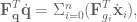
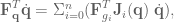
With the forces of inertia accounted for, we can now address the problem of gravity. To compensate for gravity the concept of conservation of energy (i.e. the work done by gravity is the same in all coordinate systems) will once again be pulled out. The controller operates by applying torque on joints, so it is necessary to be able to calculate the effect of gravity in joint space to cancel it out.

While the effect of gravity in joint space isn’t obvious, it is quite easily defined in Cartesian coordinates in the base frame of reference. Here, the work done by gravity is simply the summation of the distance each link’s center of mass has moved multiplied by the force of gravity. Where the force of gravity in Cartesian space is the mass of the object multiplied by -9.8m/s $^2$ along the $z$ axis, the equation for the work done by gravity is written:

$\textbf{W}_g = \Sigma^n_{i=0} (\textbf{F}_{g_i}^T \dot{\textbf{x}}_i),$

where $\textbf{F}_{g_i}$ is the force of gravity on the $i$ th arm segment. Because of the conservation of energy, the equation for work is equivalent when calculated in joint space, substituting into the above equation with the equation for work:

$\textbf{F}_\textbf{q}^T \dot{\textbf{q}} = \Sigma^n_{i=0} (\textbf{F}_{g_i}^T \dot{\textbf{x}}_i),$

and then substitute in using $\dot{\textbf{x}}_i = \textbf{J}_i(\textbf{q}) \; \dot{\textbf{q}}$ ,

$\textbf{F}_\textbf{q}^T \dot{\textbf{q}} = \Sigma^n_{i=0} (\textbf{F}_{g_i}^T \textbf{J}_i(\textbf{q}) \; \dot{\textbf{q}}),$

and cancelling out the $\dot{\textbf{q}}$ terms on both sides,

$\textbf{F}_\textbf{q}^T = \Sigma^n_{i=0} (\textbf{F}_{g_i}^T \textbf{J}_i(\textbf{q})),$

$\textbf{F}_\textbf{q} = \Sigma^n_{i=0} (\textbf{J}_i^T(\textbf{q}) \textbf{F}_{g_i}) = \textbf{g}(\textbf{q}),$

which says that to find the effect of gravity in joint space simply multiply the mass of each link by its Jacobian, multiplied by the force of gravity in $(x,y,z)$ space, and sum over each link. This summation gives the total effect of the gravity on the system.

Making a PD controller in joint space

We are now able to account for the energy in the system caused by inertia and gravity, great! Let’s use this to build a simple PD controller in joint space. Control should be very straight forward because once we cancel out the effects of gravity and inertia then we can almost pretend that the system behaves linearly. This means that we can also treat control of each of the joints independently, since their movements no longer affect one another. So in our control system we’re actually going to have a PD controller for each joint.

The above-mentioned nonlinearity that’s left in the system dynamics is due to the Coriolis and centrifugal effects. Now, these can be accounted for, but they require highly accurate model of the moments of inertia. If the moments are incorrect then the controller can actually introduce instability into the system, so it’s better if we just don’t address them.

Rewriting the system dynamics presented at the very top, in terms of acceleration gives

$\ddot{\textbf{q}} = \textbf{M}^{-1}(\textbf{q}) (\textbf{u} - \textbf{C}(\textbf{q}, \dot{\textbf{q}}) - \textbf{g}(\textbf{q})).$

Ideally, the control signal would be constructed

$\textbf{u} = (\textbf{M}(\textbf{q}) \; \ddot{\textbf{q}}_\textrm{des} + \textbf{C}(\textbf{q}, \dot{\textbf{q}}) + \textbf{g}(\textbf{q})),$

where $\ddot{\textbf{q}}_\textrm{des}$ is the desired acceleration of the system. This would result in system acceleration

$\ddot{\textbf{q}} = \textbf{M}^{-1}(\textbf{q})((\textbf{M}(\textbf{q}) \; \ddot{\textbf{q}}_\textrm{des} + \textbf{C}(\textbf{q}, \dot{\textbf{q}}) + \textbf{g}(\textbf{q})) - \textbf{C}(\textbf{q}, \dot{\textbf{q}}) - \textbf{g}(\textbf{q})),$

$\ddot{\textbf{q}} = \textbf{M}^{-1}(\textbf{q}) \textbf{M}(\textbf{q}) \; \ddot{\textbf{q}}_\textrm{des} ,$

$\ddot{\textbf{q}} = \ddot{\textbf{q}}_\textrm{des},$

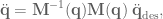
which would be ideal. As mentioned, because the Coriolis and centrifugal effects are tricky to account for we’ll leave them out, so the instead the control signal is

$\textbf{u} = (\textbf{M}(\textbf{q}) \; \ddot{\textbf{q}}_\textrm{des} + \textbf{g}(\textbf{q})).$

Using a standard PD control formula to generate the desired acceleration:

$\ddot{\textbf{q}}_\textrm{des} = k_p \; (\textbf{q}_{\textrm{des}} - \textbf{q}) + k_v \; (\dot{\textbf{q}}_{\textrm{des}} - \dot{\textbf{q}}),$

where $k_p$ and $k_v$ are our gain values, and the control signal has been fully defined:

$\textbf{u} = (\textbf{M}(\textbf{q}) \; (k_p \; (\textbf{q}_{\textrm{des}} - \textbf{q}) + k_v \; (\dot{\textbf{q}}_{\textrm{des}} - \dot{\textbf{q}})) + \textbf{g}(\textbf{q})),$

and we’ve successfully build an effective PD controller in joint space!

Conclusions

Here we looked at building a PD controller that operates in the joint space of a robotic arm that can cancel out the effects of inertia and gravity. By cancelling out the effects of inertia, we can treat control of each of the joints independently, effectively orthogonalizing their control. This makes PD control super easy, we just set up a simple controller for each joint. Also a neat thing is that all of the required calculations can be performed with algorithms of linear complexity, so it’s not a problem to do all of this super fast.

One of the finer points was that we ignored the Coriolis and centrifugal effects on the robot’s dynamics. This is because in the mass matrix model of the moments of inertia are notoriously hard to accurately capture on actual robots. Often you go based off of a CAD model of your robot and then have to do some fine-tuning by hand. So they will be unaccounted for in our control signal, but most of the time as long as you have a very short feedback loop you’ll be fine.

I am really enjoying working through this, as things build on each other so well here and we’re starting to be able to do some really interesting things with the relatively forward transformation matrices and Jacobians that we learned how to build in the previous posts. This was for a very simple robot, but excitingly the next step after this is moving on to operational space control! At last. From there, we’ll go on to look at more complex robotic situations where things like configuration redundancy are introduced and it’s not quite so straightforward.

22 thoughts on “Robot control part 3: Accounting for mass and gravity”

Pooja Voladoddi says:

March 25, 2014 at 11:21 am

Hello,

If I know the CoM of individual links , and I need to get the jacobian of the center of mass , how would I get the com of the whole robot ?

If I have a planar link , say a 2 link robot as you’ve shown, CoM (of the whole robot) would be given by summation of the two individual COMs of the links ?

[Generally ,For a rigid body one could say summation of (mass * lengths)/ summation of (masses). ]

- travisdewolf says:
  
  March 25, 2014 at 12:04 pm
  
  Yup! Exactly right, you can find the CoM of the whole robot by summing (transformations for each link’s CoM * their CoM) / sum of CoMs. There’s an illustration here: http://www.elysium-labs.com/robotics-corner/learn-robotics/biped-basics/center-of-mass/
  
  - Valentin says:
    
    May 28, 2020 at 3:43 pm
    
    Hi ! Thanks for your blog, it really helps me for my research ! The link to calculate the COM of the whole robot does not work anymore. Could you update it or just put a similar link ?
    I really need to understand clearly each step of the process to calculate the total COM, it would help ! Thanks !
  - travisdewolf says:
    
    May 28, 2020 at 3:47 pm
    
    Hi Valentin, ah that’s unfortunate. I suggest scanning through google for some more examples, I unfortunately don’t have any others off the top of my head. I did see this, though, on a cursory scan and you may find it helpful: https://www.khanacademy.org/science/physics/linear-momentum/center-of-mass/a/what-is-center-of-mass
  - Valentin says:
    
    June 1, 2020 at 9:22 am
    
    Thanks for the quick answer ! Unfortunately, what KhanAcademy shows is too trivial, I was looking to incorporate transformation matrices with the calculation of the total COM. By the way, in the answer you gave to Pooja, you said that the total COM was “(transformations for each link’s CoM * their CoM) / sum of CoMs”, but you meant “(transformations for each link’s CoM * their CoM) / sum of their masses”, right ?
Robotics_Enthusiast says:

March 29, 2014 at 4:49 pm

Hi Travis! Great posts along with great explanations!
But I think you have messed up Tcom1. The transformation matrix you have used is incorrect. I think the Rotation part of it should be
|cos(-theta0) 0 sin(-theta0) |
| 0 1 0 |
|-sin(-theta0) 0 cos(-theta0) |
Can you please check? The final value of Tcom1 is wrong anyway if you multiply the matrices given. Hope I have been of help. 🙂

- travisdewolf says:
  
  March 29, 2014 at 5:40 pm
  
  Hmm, it’s possible! There’s a lot of equations going on and I have definitely made mistakes. But I don’t think that’s going on here, if you look back at my previous post https://studywolf.wordpress.com/2013/09/02/robot-control-jacobians-velocity-and-force/ you can see how you get the answer from multiplying the matrices given. And if you check out my first one https://studywolf.wordpress.com/2013/08/21/robot-control-forward-transformation-matrices/ it shows how I came up with the rotation part for Tcom1.
  If there’s still something that catches you as wrong though please let me know! It’s important to me that all the math is correct and I really appreciate people taking the time to work through and double check everything!
  
  - Benjamin Bokser says:
    
    January 21, 2020 at 10:29 pm
    
    Hi Travis, I think the source of confusion is that here you used q1 for the rotation matrix whereas in the previous guide you used q0 for the rotation matrix. Despite them both being T1 for nearly identical arms.
Adnan Munawar says:

May 24, 2014 at 11:44 pm

Hey Travis,
Can you please clarify this equation
\textbf{W}_g = \Sigma^n_{i=0} (\textbf{F}_{g_i}^T \dot{\textbf{x}}_i)

I don’t know if you are bringing this from somewhere in the previous tutorial but isn’t the work done equal to force * distance, instead of force * velocity as shown in the equation. Am I missing something?

- travisdewolf says:
  
  May 29, 2014 at 9:14 pm
  
  Hi Adnan,
  nope you’re not missing anything from another section! Rather it’s that work is equal to force * velocity if we’re considering the work that’s done at some _instant_ of time, which we are! This is because for some instant of time the distance that you’ve move is your velocity. They talk about it a bit more here: http://en.wikipedia.org/wiki/Work_(physics)#Mathematical_calculation
  Hope that helps!
  
Robot control part 4: Operation space control | studywolf says:

March 31, 2015 at 2:55 pm

[…] in the dynamics of the system, as defined in the previous post, but ignoring the effects of gravity for now, […]

Robot control part 5: Controlling in the null space | studywolf says:

March 31, 2015 at 4:06 pm

[…] was defined in the previous post, and is defined two posts ago, and and are gain terms, usually set such that , and adding in the null space control signal and […]

jaime says:

November 17, 2015 at 8:59 am

Hi Travis!
In your last 2 equations you write that the desired acceleration are the gains values times the error of joint position and error of joint velocity.
But trying to see the physical meaning I see it should be: real acceleration (q_dot_dot) is equal to desired acceleration PLUS these gains times these errors.
Because as you described it in the last formula it would mean that when there is no error in position and velocity there is no desired acceleration.
Please see slide 8 in this presentation: http://www.in.tum.de/fileadmin/user_upload/Lehrstuehle/Lehrstuhl_XXIII/Layout/SBRML_Part2_Task_Space_Control.pdf

What do you think?

Btw Nice job! and greets 🙂

- travisdewolf says:
  
  November 17, 2015 at 10:45 pm
  
  Hi Jaime, greetings!
  
  Humm so I think there may be a bit of confusion about what the last two equations describe. The last two equations here describe the form of the control signal, not the actual dynamics of the system. When you work the control signal (which is the desired acceleration wrapped up with the gravity and inertia compensation terms) into the actual dynamics of the system (described a few lines above), then you’re right. The real acceleration of the system includes the actual dynamics of the system plus these terms added from the control signal. But as they’re written the last two equations only describe the desired control signal, not the real acceleration of the system. Does that help clarify things? 🙂
  
  In the presentation you’ve linked they’re describing the desired acceleration in operational space, and then calculating the corresponding force in operational space, and then translating that into joint torques. Here, we’re still dealing with things in joint space only, but in the next post we discuss operational space control, and you’ll see we actually end up with the same form of equation. Hope that helps! Thanks for the comment!
  
Using SymPy’s lambdify for generating transform matrices and Jacobians | studywolf says:

August 27, 2016 at 9:22 am

[…] then using our equations for calculating the system’s inertia and gravity we create our _calc_Mq and _calc_Mq_g […]

Fabian says:

March 30, 2017 at 4:40 am

Hi, first of all: great job of explaining robotic relevant topics 😉
I think that you forgot the link lengths when stating the coordinates of the respective CoMs.

- travisdewolf says:
  
  March 30, 2017 at 4:21 pm
  
  Glad you found it useful!
  
  Hummm, I’m not sure exactly where you’re referring to. After the first figure, where com_0 and com_1 are defined?
  
  - jeff says:
    
    April 19, 2017 at 7:43 pm
    
    I was wondering about the same section. For instance, if you assume your COM_0 is halfway along the 0th link, then the COM_0 X component should be something like 1/2 * L0 * cos(q0).
  - travisdewolf says:
    
    June 1, 2017 at 10:03 am
    
    Ah I see. You’re right it’s not super clear, when writing I intended that the 1/2 and 1/4 were absolute distances, not relative to the length of L0 or L1.
    Hmm, it’s on my list to do a rework of this for clarity, I’ll add this to the list of things to change! Thanks for your feedback!
adamgilesmetcalf says:

October 17, 2018 at 10:32 am

Hello Travis,

Great stuff!

At one point you say:

“Using a standard PD control formula to generate the desired acceleration:

\ddot{\textbf{q}}_\textrm{des} = k_p \; (\textbf{q}_{\textrm{des}} – \textbf{q}) + k_v \; (\dot{\textbf{q}}_{\textrm{des}} – \dot{\textbf{q}}),”

Could you point me in the direction of an article or book which can help me understand how this part works?

Thanks!
Adam.

- adamgilesmetcalf says:
  
  January 7, 2019 at 9:10 am
  
  I feel that I should specify, is there anywhere that this standard PD formula is citeable, or is it simply the design of specifically your control signal?
  
- travisdewolf says:
  
  March 5, 2019 at 3:56 pm
  
  Hi! Most any control or robotics text book will use a PD signal and can e cited. You can find it, for example, in the Introduction to Robotics textbook by John Craig (section 9.7, page 277), or in (section 10.3.1, page 239) of the Robot dynamics and control 2nd edition book by Spong et al.