Recently in my posts I’ve been using finite differences to approximate the gradient of loss functions and dynamical systems, with the intention of creating generalizable controllers that can be run on any system without having to calculate out derivatives beforehand. Finite differences is pretty much the most straight-forward way of approximating a gradient that there is: vary each parameter up and down (assuming we’re doing central differencing), one at a time, run it through your function and estimate the parameters effect on the system by calculating the difference between resulting function output. To do this requires 2 samples of the function for each parameter.
But there’s always more than one way to peel an avocado, and another approach that’s been used with much success is the Simultaneous Perturbation Stochastic Approximation (SPSA) algorithm, which was developed by Dr. James Spall (link to overview paper). SPSA is a method of gradient approximation, like finite differences, but, critically, the difference is that it varies all of the parameters at once, rather than one at a time. As a result, you can get an approximation of the gradient with far fewer samples from the system, and also when you don’t have explicit control over your samples (i.e. the ability to vary each parameter one at a time).
Gradient approximation
Given some function 


where 
And that’s how we’ve calculated it before, estimating the gradient of a single parameter at a time. But, we can rewrite this for a set perturbations ![\Delta \textbf{X} = [\Delta\textbf{x}_0, ... , \Delta\textbf{x}_N]^T](https://s0.wp.com/latex.php?latex=%5CDelta+%5Ctextbf%7BX%7D+%3D+%5B%5CDelta%5Ctextbf%7Bx%7D_0%2C+...+%2C+%5CDelta%5Ctextbf%7Bx%7D_N%5D%5ET&bg=ffffff&fg=555555&s=0&c=20201002)

where
![\textbf{F} = [\frac{\textbf{f}(\textbf{x} + \Delta \textbf{x}_0) - \textbf{f}(\textbf{x} - \Delta \textbf{x}_0)}{2}, ... , \frac{\textbf{f}(\textbf{x} + \Delta \textbf{x}_0) - \textbf{f}(\textbf{x}_N - \Delta \textbf{x}_N)}{2}]^T](https://s0.wp.com/latex.php?latex=%5Ctextbf%7BF%7D+%3D+%5B%5Cfrac%7B%5Ctextbf%7Bf%7D%28%5Ctextbf%7Bx%7D+%2B+%5CDelta+%5Ctextbf%7Bx%7D_0%29+-+%5Ctextbf%7Bf%7D%28%5Ctextbf%7Bx%7D+-+%5CDelta+%5Ctextbf%7Bx%7D_0%29%7D%7B2%7D%2C+...+%2C+%5Cfrac%7B%5Ctextbf%7Bf%7D%28%5Ctextbf%7Bx%7D+%2B+%5CDelta+%5Ctextbf%7Bx%7D_0%29+-+%5Ctextbf%7Bf%7D%28%5Ctextbf%7Bx%7D_N+-+%5CDelta+%5Ctextbf%7Bx%7D_N%29%7D%7B2%7D%5D%5ET&bg=ffffff&fg=555555&s=0&c=20201002)
which works as long as 


By rewriting the above, and getting rid of the inverse by moving

Now, the standard trick to move a matrix that’s not square is to just make it square by multiplying it by its transpose to get a square matrix, and then the whole thing by the inverse:


Alright! Now we’re comfortable with this characterization of gradient approximation using a form that works with non-square perturbation matrices.
Again, in FDSA, we only vary one parameter at a time. This means that there will only ever be one non-zero entry per row of
Gradient approximation to estimate 

This paper, by Drs. Jan Peters and Stepfan Schaal, is where I first stumbled across the above formulation of gradient approximation and read about SPSA (side note: I really recommend reading instead the Scholarpedia article on policy gradients, because it has fixes to a couple notation mistakes from the paper). Reading about this I thought, oh interesting, an alternative to FDSA for gradient approximation, let’s see how it well it does replacing FDSA in a linear quadratic regulator (LQR).
Implementing this was pretty simple. Just had to modify the calc_derivs function, which I use to estimate the derivative of the arm with respect to the state and control signal, in my LQR controller code by changing from standard finite differences to simultaneous perturbation:
def calc_derivs(self, x, u):
    """" calculate gradient of plant dynamics using Simultaneous
    Perturbation Stochastic Approximation (SPSA). Implemented
    based on (Peters & Schaal, 2008).

    x np.array: the state of the system
    u np.array: the control signal
    """
    # Initialization and coefficient selection
    num_iters = 20

    eps = 1e-4
    delta_K = None
    delta_J = None
    for ii in range(num_iters):
        # Generation of simultaneous perturbation vector
        # choose each component from a Bernoulli +-1 distribution
        # with probability of .5 for each +-1 outcome.
        delta_k = np.random.choice([-1,1],
                                   size=len(x) + len(u),
                                   p=[.5, .5])
        # Function evaluations
        inc_x = np.copy(x) + eps * delta_k[:len(x)]
        inc_u = np.copy(u) + eps * delta_k[len(x):]
        state_inc = self.plant_dynamics(inc_x, inc_u)
        dec_x = np.copy(x) - eps * delta_k[:len(x)]
        dec_u = np.copy(u) - eps * delta_k[len(x):]
        state_dec = self.plant_dynamics(dec_x, dec_u)

        delta_j = ((state_inc - state_dec) /
                        (2.0 * eps)).reshape(-1)

        # Track delta_k and delta_j
        delta_K = delta_k if delta_K is None else \
            np.vstack([delta_K, delta_k])
        delta_J =  delta_j if delta_J is None else \
            np.vstack([delta_J, delta_j])

    f_xu = np.dot(np.linalg.pinv(np.dot(delta_K.T, delta_K)),
            np.dot(delta_K.T, delta_J))
    f_x = f_xu[:len(x)]
    f_u = f_xu[len(x):]

    return f_x.T , f_u.T
A couple notes about the above code. First, you’ll notice that the f_x and f_b matrices are both calculated at the same time. That’s pretty slick! And that calculation for f_xu is just a straight implementation of the matrix form of gradient approximation, where I’ve arranged things so that f_x is in the top part and f_u is in the lower part.
The second thing is that the perturbation vector delta_k is generated from a Bernoulli distribution. The reason behind this is that we want to have a bunch of different samples that pretty reasonably spread the state space and move all the parameters independently. Making each perturbation some distance times -1 or 1 is an easy way to achieve this.
Thirdly, there’s the num_iters variable. This is a very important variable, as it dictates how many random samples of our system we take before we estimate the gradient. I’ve found that to get this to work for both the 2-link arm and the more complex 3-link arm, it needs to be at least 20. Or else things explode and die horribly. Just…horribly.
OK let’s look at the results:


The first thing to notice is that I’ve finally discovered the Seaborn plotting package. The second is that SPSA does as well as FDSA.
You may ask: Is there any difference? Well, if we time these functions, on my lil’ laptop, for the 2-link arm it takes SPSA approximately 2.0ms, but it takes FDSA only 0.8ms. So for the same performance the SPSA is taking almost 3 times as long to run. Why? This boils down to how many times the system dynamics need to be sampled by each algorithm to get a good approximation of the gradient. For a 2-link arm, FDSA has 6 parameters (

For the 3-link arm, SPSA took about 3.1ms on average and FDSA (which must now perform 18 samples of the dynamics) still only 2.1ms. So number of samples isn’t the only cause of time difference between these two algorithms. SPSA needs to perform that a few more matrix operations, including a matrix inverse, which is expensive, while FDSA can calculate the gradient of each parameter individually, which is much less expensive.
OK so SPSA not really impressive here. BUT! As I discovered, there are other means of employing SPSA.
Gradient approximation to optimize the control signal directly
In the previous set up we were using SPSA to estimate the gradient of the system under control, and then we used that gradient to calculate a control signal that minimized the loss function (as specified inside the LQR). This is one way to use gradient approximation methods. Another way to use these methods is approximate the gradient of the loss function directly, and use that information to iteratively calculate a control signal that minimizes the loss function. This second application is the primary use of the SPSA algorithm, and is what’s described by Dr. Spall in his overview paper.
In this application, the algorithm works like this:
- start with initial input to system
- perturb input and simulate results
- observe loss function and calculate gradient
- update input to system
- repeat to convergence
Because in this approach we’re iteratively optimizing the input using our gradient estimation, having a noisy estimate is no longer a death sentence, as it was in the LQR. If we update our input to the system with several noisy gradient estimates the noise will essentially just cancel itself out. This means that SPSA now has a powerful advantage over FDSA: Since in SPSA we vary all parameters at once, only 2 samples of the loss function are used to estimate the gradient, regardless of the number of parameters. In contrast, FDSA needs to sample the loss function twice for every input parameter. Here’s a picture from (Spall, 1998) that shows the two running against each other to optimize a 2D problem:

This gets across that even though SPSA bounces around more, they both reach the solution in the same number of steps. And, in general, this is the case, as Dr. Spall talks about in the paper. There’s also a couple more details of the algorithm, so let’s look at it in detail. Here’s the code, which is just a straight translation into Python out of the description in Dr. Spall’s paper:
# Step 1: Initialization and coefficient selection
max_iters = 5
converge_thresh = 1e-5

alpha = 0.602 # from (Spall, 1998)
gamma = 0.101
a = .101 # found empirically using HyperOpt
A = .193
c = .0277

delta_K = None
delta_J = None
u = np.copy(self.u) if self.u is not None \
        else np.zeros(self.arm.DOF)
for k in range(max_iters):
    ak = a / (A + k + 1)**alpha
    ck = c / (k + 1)**gamma

    # Step 2: Generation of simultaneous perturbation vector
    # choose each component from a bernoulli +-1 distribution with
    # probability of .5 for each +-1 outcome.
    delta_k = np.random.choice([-1,1], size=arm.DOF, p=[.5, .5])

    # Step 3: Function evaluations
    inc_u = np.copy(u) + ck * delta_k
    cost_inc = self.cost(np.copy(state), inc_u)
    dec_u = np.copy(u) - ck * delta_k
    cost_dec = self.cost(np.copy(state), dec_u)

    # Step 4: Gradient approximation
    gk = np.dot((cost_inc - cost_dec) / (2.0*ck), delta_k)

    # Step 5: Update u estimate
    old_u = np.copy(u)
    u -= ak * gk

    # Step 6: Check for convergence
    if np.sum(abs(u - old_u)) < converge_thresh:
        break
The main as-of-yet-unexplained parts of this code are the alpha, gamma, a, A, and c variables. What’s their deal?
Looking inside the loop, we can see that ck controls the magnitude of our perturbations. Looking a little further down, ak is just the learning rate. And all of those other parameters are just involved in shaping the trajectories that ak and ck follow through iterations, which is a path towards zero. So the first steps and perturbations are the biggest, and each successively becomes smaller as the iteration count increases.
There are a few heuristics that Dr. Spall goes over, but there aren’t any hard and fast rules for setting a, A, and c. Here, I just used HyperOpt to find some values that worked pretty well for this particular problem.
The FDSA version of this is also very straight-forward:
# Step 1: Initialization and coefficient selection
max_iters = 10
converge_thresh = 1e-5

eps = 1e-4
u = np.copy(self.u) if self.u is not None \
        else np.zeros(self.arm.DOF)
for k in range(max_iters):

    gk = np.zeros(u.shape)
    for ii in range(gk.shape[0]):
        # Step 2: Generate perturbations one parameter at a time
        inc_u = np.copy(u)
        inc_u[ii] += eps
        dec_u = np.copy(u)
        dec_u -= eps

        # Step 3: Function evaluation
        cost_inc = self.cost(np.copy(state), inc_u)
        cost_dec = self.cost(np.copy(state), dec_u)

        # Step 4: Gradient approximation
        gk[ii] = (cost_inc - cost_dec) / (2.0 * eps)

    old_u = np.copy(u)
    # Step 5: Update u estimate
    u -= 1e-5 * gk

    # Step 6: Check for convergence
    if np.sum(abs(u - old_u)) < converge_thresh:
        break
You’ll notice that in both the SPSA and FDSA code we’re no longer sampling plant_dynamics, we’re instead sampling cost, a loss function I defined. From just my experience playing around with these algorithms a bit, getting the loss function to be appropriate and give the desired behaviour is definitely a bit of an art. It feels like much more of an art than in other controllers I’ve coded, but that could just be me.
The cost function that I’m using is pretty much the first thing you’d think of. It penalizes distance to target and having non-zero velocity. Getting the weighting between distance to target and velocity set up so that the arm moves to the target but also doesn’t overshoot definitely took a bit of trial and error, er, I mean empirical analysis. Here’s the cost function that I found worked pretty well, note that I had to make special cases for the different arms:
 def cost(self, x, u):
        dt = .1 if self.arm.DOF == 3 else .01
        next_x = self.plant_dynamics(x, u, dt=dt)
        vel_gain = 100 if self.arm.DOF == 3 else 10
        return (np.sqrt(np.sum((self.arm.x - self.target)**2)) * 1000 \
                + np.sum((next_x[self.arm.DOF:])**2) * vel_gain)
So that’s all the code, let’s look at the results!


For these results, I used a max of 10 iterations for optimizing the control signal. I was definitely surprised by the quality of the results, especially for the 3-link arm, compared to the results generated by a standard LQR controller. Although I need to note, again, that it was a fair bit of me playing around with the exact cost function to get these results. Lots of empirical analysis.
The two controllers generate results that are identical to visual inspection. However, especially in the 3-link arm, the time required to run the FDSA was significantly longer than the SPSA controller. It took approximately 140ms for the SPSA controller to run a single loop, but took FDSA on average 700ms for a single loop of calculating the control signal. Almost 5 times as long! For the same results! In directly optimizing the control signal, SPSA gets a big win over standard FDSA. So, if you’re looking to directly optimize over a loss function, SPSA is probably the way you want to go.
Conclusions
First off, I thought it was really neat to directly apply gradient approximation methods to optimizing the control signal. It’s something I haven’t tried before, but definitely makes sense, and can generate some really nice results when tuned properly. Automating the tuning is definitely I’ll be discussing in future posts, because doing it by hand takes a long time and is annoying.
In the LQR, the gradient approximation was best done by the FDSA. I think the main reasons for this is that in solving for the control signal the LQR algorithm uses matrix inverses, and any errors in the linear approximations to the dynamics are going to be amplified quite a bit. If I did anything less than 10-15 iterations (20 for the 3-link arm) in the SPSA approximation then things exploded. Also, here the SPSA algorithm required a matrix inverse, where the FDSA didn’t. This is because we only varied one parameter at a time in FDSA, and the effects of changing each was isolated. In the SPSA case, we had to consider the changes across all the variables and the resulting effects all at once, essentially noting which variables changed by how much and the changes in each case, and averaging. Here, even with the more complex 3-link arm, FDSA was faster, so I’m going to stick with it in my LQR and iLQR implementations.
In the direct control signal optimization SPSA beat the pants off of FDSA. It was almost 5 times faster for control of the 3-link arm. This was, again, because in this case we could use noisy samples of the gradient of the loss function and relied on noise to cancel itself out as we iterated. So we only needed 2 samples of the loss function in SPSA, where in FDSA we needed 2*num_parameters. And although this generated pretty good results I would definitely be hesitant against using this for any more complicated systems, because tuning that cost function to get out a good trajectory was a pain. If you’re interested in playing around with this, you can check out the code for the gradient controllers up on my GitHub.

 is joint angle acceleration,
  is a function describing the Coriolis and centrifugal effects,
  is the effect of gravity in joint space, and
  is the mass matrix of the system in joint space.
 is not sufficient, because a lot of the dynamics affecting acceleration aren’t accounted for. In this section an effective PD controller operating in joint space will be developed that will allow for more precise control by cancelling out unwanted acceleration terms. To do this the effects of inertia and gravity need to be calculated.
 plane, with the
  axis extending into the picture where the yellow circles represent each links centre-of-mass (COM). The position of each link is COM is defined relative to that link’s reference frame, and the goal is to figure out how much each link’s mass will affect the system dynamics.
![\textrm{com}_0 = \left[ \begin{array}{c} \frac{1}{2}cos(q_0) \\ 0 \\ \frac{1}{2}sin(q_0) \end{array} \right], \;\;\;\; \textrm{com}_1 = \left[ \begin{array}{c} \frac{1}{4}cos(q_1) \\ 0 \\ \frac{1}{4}sin(q_1) \end{array} \right].](https://s0.wp.com/latex.php?latex=%5Ctextrm%7Bcom%7D_0+%3D+%5Cleft%5B+%5Cbegin%7Barray%7D%7Bc%7D+%5Cfrac%7B1%7D%7B2%7Dcos%28q_0%29+%5C%5C+0+%5C%5C+%5Cfrac%7B1%7D%7B2%7Dsin%28q_0%29+%5Cend%7Barray%7D+%5Cright%5D%2C+%5C%3B%5C%3B%5C%3B%5C%3B+%5Ctextrm%7Bcom%7D_1+%3D+%5Cleft%5B+%5Cbegin%7Barray%7D%7Bc%7D+%5Cfrac%7B1%7D%7B4%7Dcos%28q_1%29+%5C%5C+0+%5C%5C+%5Cfrac%7B1%7D%7B4%7Dsin%28q_1%29+%5Cend%7Barray%7D+%5Cright%5D.&bg=ffffff&fg=555555&s=0&c=20201002)
![^1_0\textbf{T} = \left[ \begin{array}{cccc} cos(q_1) & 0 & -sin(q_1) & L_0 cos(q_0) \\ 0 & 1 & 0 & 0 \\ sin(q_1) & 0 & cos(q_1) & L_0 sin(q_0) \\ 0 & 0 & 0 & 1 \end{array} \right].](https://s0.wp.com/latex.php?latex=%5E1_0%5Ctextbf%7BT%7D+%3D+%5Cleft%5B+%5Cbegin%7Barray%7D%7Bcccc%7D+cos%28q_1%29+%26+0+%26+-sin%28q_1%29+%26+L_0+cos%28q_0%29+%5C%5C+0+%26+1+%26+0+%26+0+%5C%5C+sin%28q_1%29+%26+0+%26+cos%28q_1%29+%26+L_0+sin%28q_0%29+%5C%5C+0+%26+0+%26+0+%26+1+%5Cend%7Barray%7D+%5Cright%5D.&bg=ffffff&fg=555555&s=0&c=20201002)
 to transform the
  gives
gives![^1_0\textbf{T} \; \textrm{com}_1 = \left[ \begin{array}{cccc} cos(q_1) & 0 & -sin(q_1) & L_0 cos(q_0) \\ 0 & 1 & 0 & 0 \\ sin(q_1) & 0 & cos(q_1) & L_0 sin(q_0) \\ 0 & 0 & 0 & 1 \end{array} \right] \; \; \left[ \begin{array}{c} \frac{1}{4}cos(q_1) \\ 0 \\ \frac{1}{4}sin(q_1) \\ 1 \end{array} \right]](https://s0.wp.com/latex.php?latex=%5E1_0%5Ctextbf%7BT%7D+%5C%3B+%5Ctextrm%7Bcom%7D_1+%3D+%5Cleft%5B+%5Cbegin%7Barray%7D%7Bcccc%7D+cos%28q_1%29+%26+0+%26+-sin%28q_1%29+%26+L_0+cos%28q_0%29+%5C%5C+0+%26+1+%26+0+%26+0+%5C%5C+sin%28q_1%29+%26+0+%26+cos%28q_1%29+%26+L_0+sin%28q_0%29+%5C%5C+0+%26+0+%26+0+%26+1+%5Cend%7Barray%7D+%5Cright%5D+%5C%3B+%5C%3B+%5Cleft%5B+%5Cbegin%7Barray%7D%7Bc%7D+%5Cfrac%7B1%7D%7B4%7Dcos%28q_1%29+%5C%5C+0+%5C%5C+%5Cfrac%7B1%7D%7B4%7Dsin%28q_1%29+%5C%5C+1+%5Cend%7Barray%7D+%5Cright%5D&bg=ffffff&fg=555555&s=0&c=20201002)
![^1_0\textbf{T} \; \textrm{com}_1 = \left[ \begin{array}{c} L_0 cos(q_0) + \frac{1}{4}cos(q_0 + q_1) \\ 0 \\ L_0 sin(q_0) + \frac{1}{4} cos(q_0 + q_1) \\ 1 \end{array} \right].](https://s0.wp.com/latex.php?latex=%5E1_0%5Ctextbf%7BT%7D+%5C%3B+%5Ctextrm%7Bcom%7D_1+%3D+%5Cleft%5B+%5Cbegin%7Barray%7D%7Bc%7D+L_0+cos%28q_0%29+%2B+%5Cfrac%7B1%7D%7B4%7Dcos%28q_0+%2B+q_1%29+%5C%5C+0+%5C%5C+L_0+sin%28q_0%29+%2B+%5Cfrac%7B1%7D%7B4%7D+cos%28q_0+%2B+q_1%29+%5C%5C+1+%5Cend%7Barray%7D+%5Cright%5D.&bg=ffffff&fg=555555&s=0&c=20201002)
 .
.![\textbf{J}_0 = \left[ \begin{array}{cc} -\frac{1}{2}sin(q_0) & 0 \\ 0 & 0 \\ \frac{1}{2} cos(q_0) & 0 \\ 0 & 0 \\ 1 & 0 \\ 0 & 0 \end{array} \right]](https://s0.wp.com/latex.php?latex=%5Ctextbf%7BJ%7D_0+%3D+%5Cleft%5B+%5Cbegin%7Barray%7D%7Bcc%7D+-%5Cfrac%7B1%7D%7B2%7Dsin%28q_0%29+%26+0+%5C%5C+0+%26+0+%5C%5C+%5Cfrac%7B1%7D%7B2%7D+cos%28q_0%29+%26+0+%5C%5C+0+%26+0+%5C%5C+1+%26+0+%5C%5C+0+%26+0+%5Cend%7Barray%7D+%5Cright%5D&bg=ffffff&fg=555555&s=0&c=20201002)
![\textbf{J}_1 = \left[ \begin{array}{cc} -L_0sin(q_0) -\frac{1}{4}sin(\theta_0 + q_1) & -\frac{1}{4} sin(q_0 + \theta_1) \\ 0 & 0 \\ L_0 cos(q_0) + \frac{1}{4}cos(q_0 + q_1) & \frac{1}{4} cos(q_0 +q_1) \\ 0 & 0 \\ 1 & 1 \\ 0 & 0 \end{array} \right]](https://s0.wp.com/latex.php?latex=%5Ctextbf%7BJ%7D_1+%3D+%5Cleft%5B+%5Cbegin%7Barray%7D%7Bcc%7D+-L_0sin%28q_0%29+-%5Cfrac%7B1%7D%7B4%7Dsin%28%5Ctheta_0+%2B+q_1%29+%26+-%5Cfrac%7B1%7D%7B4%7D+sin%28q_0+%2B+%5Ctheta_1%29+%5C%5C+0+%26+0+%5C%5C+L_0+cos%28q_0%29+%2B+%5Cfrac%7B1%7D%7B4%7Dcos%28q_0+%2B+q_1%29+%26+%5Cfrac%7B1%7D%7B4%7D+cos%28q_0+%2Bq_1%29+%5C%5C+0+%26+0+%5C%5C+1+%26+1+%5C%5C+0+%26+0+%5Cend%7Barray%7D+%5Cright%5D&bg=ffffff&fg=555555&s=0&c=20201002) .
.
 is the mass matrix of the system, with the subscript
  is a velocity vector, where
 ![\dot{\textbf{x}} = \left[ \begin{array}{c} \dot{x} \\ \dot{y} \\ \dot{z} \\ \dot{\omega_x} \\ \dot{\omega_y} \\ \dot{\omega_z} \end{array} \right],](https://s0.wp.com/latex.php?latex=%5Cdot%7B%5Ctextbf%7Bx%7D%7D+%3D+%5Cleft%5B+%5Cbegin%7Barray%7D%7Bc%7D+%5Cdot%7Bx%7D+%5C%5C+%5Cdot%7By%7D+%5C%5C+%5Cdot%7Bz%7D+%5C%5C+%5Cdot%7B%5Comega_x%7D+%5C%5C+%5Cdot%7B%5Comega_y%7D+%5C%5C+%5Cdot%7B%5Comega_z%7D+%5Cend%7Barray%7D+%5Cright%5D%2C&bg=ffffff&fg=555555&s=0&c=20201002)
![\textbf{M}_{\textbf{x}_i} (\textbf{q})= \left[ \begin{array}{cccccc} m_i & 0 & 0 & 0 & 0 & 0 \\ 0 & m_i & 0 & 0 & 0 & 0 \\ 0 & 0 & m_i & 0 & 0 & 0 \\ 0 & 0 & 0 & I_{xx} & I_{xy} & I_{xz} \\ 0 & 0 & 0 & I_{yx} & I_{yy} & I_{yz} \\ 0 & 0 & 0 & I_{zx} & I_{zy} & I_{zz} \end{array} \right],](https://s0.wp.com/latex.php?latex=%5Ctextbf%7BM%7D_%7B%5Ctextbf%7Bx%7D_i%7D+%28%5Ctextbf%7Bq%7D%29%3D+%5Cleft%5B+%5Cbegin%7Barray%7D%7Bcccccc%7D+m_i+%26+0+%26+0+%26+0+%26+0+%26+0+%5C%5C+0+%26+m_i+%26+0+%26+0+%26+0+%26+0+%5C%5C+0+%26+0+%26+m_i+%26+0+%26+0+%26+0+%5C%5C+0+%26+0+%26+0+%26+I_%7Bxx%7D+%26+I_%7Bxy%7D+%26+I_%7Bxz%7D+%5C%5C+0+%26+0+%26+0+%26+I_%7Byx%7D+%26+I_%7Byy%7D+%26+I_%7Byz%7D+%5C%5C+0+%26+0+%26+0+%26+I_%7Bzx%7D+%26+I_%7Bzy%7D+%26+I_%7Bzz%7D+%5Cend%7Barray%7D+%5Cright%5D%2C&bg=ffffff&fg=555555&s=0&c=20201002)
 is the mass of COM
  , and the
  terms are the moments of inertia, which define the object’s resistance to change in angular velocity about the axes, the same way that the mass element defines the object’s resistance to changes in linear velocity.
 ,
,
 terms outside the summation,

 denotes the inertia matrix in joint space.
 along the
  axis, the equation for the work done by gravity is written:
 is the force of gravity on the
 ,
,


 space, and sum over each link. This summation gives the total effect of the gravity on the system.

 is the desired acceleration of the system. This would result in system acceleration


 and
and  are our gain values, and the control signal has been fully defined:
 ). The Jacobian for this system relates how movement of the elements of
  ,
, , multiplied by the joint angle velocity.
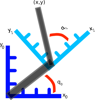
![\textbf{q} = [q_0, q_1]^T](https://s0.wp.com/latex.php?latex=%5Ctextbf%7Bq%7D+%3D+%5Bq_0%2C+q_1%5D%5ET&bg=ffffff&fg=555555&s=0&c=20201002) , and end-effector position be denoted
, and end-effector position be denoted ![\textbf{x} = [x, y, 0]^T](https://s0.wp.com/latex.php?latex=%5Ctextbf%7Bx%7D+%3D+%5Bx%2C+y%2C+0%5D%5ET&bg=ffffff&fg=555555&s=0&c=20201002) .
.
 is work,
  is force, and
  is velocity.
 is power.

 is the force applied to the hand, and
 is the torque applied to the joints, and


 is the Jacobian for the end-effector of the robot, and
  represents the forces in joint-space that affect movement of the hand. This says that not only does the Jacobian relate velocity from one state-space representation to another, it can also be used to calculate what the forces in joint space should be to effect a desired set of forces in end-effector space.
 . However will we do it? Well, we know the distances from the shoulder to the elbow, and elbow to the wrist, as well as the joint angles, and we’re interested in finding out where the end-effector is relative to a base coordinate frame…OH MAYBE we should use those forward transformation matrices from the previous post. Let’s do it!
![^1_0\textbf{R} = \left[ \begin{array}{ccc} cos(q_0) & -sin(q_0) & 0 \\ sin(q_0) & cos(q_0) & 0 \\ 0 & 0 & 1 \end{array} \right].](https://s0.wp.com/latex.php?latex=%5E1_0%5Ctextbf%7BR%7D+%3D+%5Cleft%5B+%5Cbegin%7Barray%7D%7Bccc%7D+cos%28q_0%29+%26+-sin%28q_0%29+%26+0+%5C%5C+sin%28q_0%29+%26+cos%28q_0%29+%26+0+%5C%5C+0+%26+0+%26+1+%5Cend%7Barray%7D+%5Cright%5D.&bg=ffffff&fg=555555&s=0&c=20201002)
 and an angle
  the
the  position of the end point is defined
  , and the
  . The arm is operating in the
  plane, so the
 ![^1_0\textbf{D} = \left[ \begin{array}{c} L_0 cos(q_0) \\ L_0 sin(q_0) \\ 0 \end{array} \right].](https://s0.wp.com/latex.php?latex=%5E1_0%5Ctextbf%7BD%7D+%3D+%5Cleft%5B+%5Cbegin%7Barray%7D%7Bc%7D+L_0+cos%28q_0%29+%5C%5C+L_0+sin%28q_0%29+%5C%5C+0+%5Cend%7Barray%7D+%5Cright%5D.+&bg=ffffff&fg=555555&s=0&c=20201002)
![^1_0\textbf{T} = \left[ \begin{array}{cc} ^1_0\textbf{R} & ^1_0\textbf{D} \\ \textbf{0} & \textbf{1} \end{array} \right] = \left[ \begin{array}{cccc} cos(q_0) & -sin(q_0) & 0 & L_0 cos(q_0) \\ sin(q_0) & cos(q_0) & 0 & L_0 sin(q_0)\\ 0 & 0 & 1 & 0 \\ 0 & 0 & 0 & 1 \end{array} \right],](https://s0.wp.com/latex.php?latex=%5E1_0%5Ctextbf%7BT%7D+%3D+%5Cleft%5B+%5Cbegin%7Barray%7D%7Bcc%7D+%5E1_0%5Ctextbf%7BR%7D+%26+%5E1_0%5Ctextbf%7BD%7D+%5C%5C+%5Ctextbf%7B0%7D+%26+%5Ctextbf%7B1%7D+%5Cend%7Barray%7D+%5Cright%5D+%3D+%5Cleft%5B+%5Cbegin%7Barray%7D%7Bcccc%7D+cos%28q_0%29+%26+-sin%28q_0%29+%26+0+%26+L_0+cos%28q_0%29+%5C%5C+sin%28q_0%29+%26+cos%28q_0%29+%26+0+%26+L_0+sin%28q_0%29%5C%5C+0+%26+0+%26+1+%26+0+%5C%5C+0+%26+0+%26+0+%26+1+%5Cend%7Barray%7D+%5Cright%5D%2C&bg=ffffff&fg=555555&s=0&c=20201002)
 and the length of second arm segment,
  :
:![\textbf{x} = \left[ \begin{array}{c} L_1 cos(q_1) \\ L_1 sin(q_1) \\ 0 \\ 1 \end{array} \right].](https://s0.wp.com/latex.php?latex=%5Ctextbf%7Bx%7D+%3D+%5Cleft%5B+%5Cbegin%7Barray%7D%7Bc%7D+L_1+cos%28q_1%29+%5C%5C+L_1+sin%28q_1%29+%5C%5C+0+%5C%5C+1+%5Cend%7Barray%7D+%5Cright%5D.+&bg=ffffff&fg=555555&s=0&c=20201002)
![^1_0\textbf{T} \; \textbf{x} = \left[ \begin{array}{cccc} cos(q_0) & -sin(q_0) & 0 & L_0 cos(q_0) \\ sin(q_0) & cos(q_0) & 0 & L_0 sin(q_0)\\ 0 & 0 & 1 & 0 \\ 0 & 0 & 0 & 1 \end{array} \right] \; \left[ \begin{array}{c} L_1 cos(q_1) \\ L_1 sin(q_1) \\ 0 \\ 1 \end{array} \right],](https://s0.wp.com/latex.php?latex=%5E1_0%5Ctextbf%7BT%7D+%5C%3B+%5Ctextbf%7Bx%7D+%3D+%5Cleft%5B+%5Cbegin%7Barray%7D%7Bcccc%7D+cos%28q_0%29+%26+-sin%28q_0%29+%26+0+%26+L_0+cos%28q_0%29+%5C%5C+sin%28q_0%29+%26+cos%28q_0%29+%26+0+%26+L_0+sin%28q_0%29%5C%5C+0+%26+0+%26+1+%26+0+%5C%5C+0+%26+0+%26+0+%26+1+%5Cend%7Barray%7D+%5Cright%5D+%5C%3B+%5Cleft%5B+%5Cbegin%7Barray%7D%7Bc%7D+L_1+cos%28q_1%29+%5C%5C+L_1+sin%28q_1%29+%5C%5C+0+%5C%5C+1+%5Cend%7Barray%7D+%5Cright%5D%2C&bg=ffffff&fg=555555&s=0&c=20201002)
![^1_0\textbf{T} \textbf{x} = \left[ \begin{array}{c} L_1 cos(q_0) cos(q_1) - L_1 sin(q_0) sin(q_1) + L_0 cos(q_0) \\ L_1 sin(q_0) cos(q_1) + L_1 cos(q_0) sin(q_1) + L_0 sin(q_0) \\ 0 \\ 1 \end{array} \right]](https://s0.wp.com/latex.php?latex=%5E1_0%5Ctextbf%7BT%7D+%5Ctextbf%7Bx%7D+%3D+%5Cleft%5B+%5Cbegin%7Barray%7D%7Bc%7D+L_1+cos%28q_0%29+cos%28q_1%29+-+L_1+sin%28q_0%29+sin%28q_1%29+%2B+L_0+cos%28q_0%29+%5C%5C+L_1+sin%28q_0%29+cos%28q_1%29+%2B+L_1+cos%28q_0%29+sin%28q_1%29+%2B+L_0+sin%28q_0%29+%5C%5C+0+%5C%5C+1+%5Cend%7Barray%7D+%5Cright%5D&bg=ffffff&fg=555555&s=0&c=20201002)


![\left[ \begin{array}{c} L_0 cos(q_0) + L_1 cos(q_0 + q_1) \\ L_0 sin(q_0) + L_1 sin(q_0 + q_1) \\ 0 \end{array} \right],](https://s0.wp.com/latex.php?latex=%5Cleft%5B+%5Cbegin%7Barray%7D%7Bc%7D+L_0+cos%28q_0%29+%2B+L_1+cos%28q_0+%2B+q_1%29+%5C%5C+L_0+sin%28q_0%29+%2B+L_1+sin%28q_0+%2B+q_1%29+%5C%5C+0+%5Cend%7Barray%7D+%5Cright%5D%2C&bg=ffffff&fg=555555&s=0&c=20201002)
![\left[ \begin{array}{c} \omega_x \\ \omega_y \\ \omega_z \end{array} \right] = \left[ \begin{array}{c} 0 \\ 0 \\ q_0 + q_1 \end{array} \right],](https://s0.wp.com/latex.php?latex=%5Cleft%5B+%5Cbegin%7Barray%7D%7Bc%7D+%5Comega_x+%5C%5C+%5Comega_y+%5C%5C+%5Comega_z+%5Cend%7Barray%7D+%5Cright%5D+%3D+%5Cleft%5B+%5Cbegin%7Barray%7D%7Bc%7D+0+%5C%5C+0+%5C%5C+q_0+%2B+q_1+%5Cend%7Barray%7D+%5Cright%5D%2C&bg=ffffff&fg=555555&s=0&c=20201002)
 denotes angular rotation. If the first joint had been rotating in a different plane, e.g. in the
  plane around the
 ![\left[ \begin{array}{c} \omega_x \\ \omega_y \\ \omega_z \end{array} \right] = \left[ \begin{array}{c} 0 \\ q_0 \\ q_1 \end{array} \right].](https://s0.wp.com/latex.php?latex=%5Cleft%5B+%5Cbegin%7Barray%7D%7Bc%7D+%5Comega_x+%5C%5C+%5Comega_y+%5C%5C+%5Comega_z+%5Cend%7Barray%7D+%5Cright%5D+%3D+%5Cleft%5B+%5Cbegin%7Barray%7D%7Bc%7D+0+%5C%5C+q_0+%5C%5C+q_1+%5Cend%7Barray%7D+%5Cright%5D.&bg=ffffff&fg=555555&s=0&c=20201002)
 and
and  , representing the linear and angular velocity, respectively, of the end-effector.
![\textbf{J}_v(\textbf{q}) = \left[ \begin{array}{cc} \frac{\partial x}{\partial q_0} & \frac{\partial x}{\partial q_1} \\ \frac{\partial y}{\partial q_0} & \frac{\partial y}{\partial q_1} \\ \frac{\partial z}{\partial q_0} & \frac{\partial z}{\partial q_1} \end{array} \right] = \left[ \begin{array}{cc} -L_0 sin(q_0) - L_1 sin(q_0 + q_1) & - L_1 sin(q_0 + q_1) \\ L_0 cos(q_0) + L_1 cos(q_0 + q_1) & L_1 cos(q_0 + q_1) \\ 0 & 0 \end{array} \right].](https://s0.wp.com/latex.php?latex=%5Ctextbf%7BJ%7D_v%28%5Ctextbf%7Bq%7D%29+%3D+%5Cleft%5B+%5Cbegin%7Barray%7D%7Bcc%7D+%5Cfrac%7B%5Cpartial+x%7D%7B%5Cpartial+q_0%7D+%26+%5Cfrac%7B%5Cpartial+x%7D%7B%5Cpartial+q_1%7D+%5C%5C+%5Cfrac%7B%5Cpartial+y%7D%7B%5Cpartial+q_0%7D+%26+%5Cfrac%7B%5Cpartial+y%7D%7B%5Cpartial+q_1%7D+%5C%5C+%5Cfrac%7B%5Cpartial+z%7D%7B%5Cpartial+q_0%7D+%26+%5Cfrac%7B%5Cpartial+z%7D%7B%5Cpartial+q_1%7D+%5Cend%7Barray%7D+%5Cright%5D+%3D+%5Cleft%5B+%5Cbegin%7Barray%7D%7Bcc%7D+-L_0+sin%28q_0%29+-+L_1+sin%28q_0+%2B+q_1%29+%26+-+L_1+sin%28q_0+%2B+q_1%29+%5C%5C+L_0+cos%28q_0%29+%2B+L_1+cos%28q_0+%2B+q_1%29+%26+L_1+cos%28q_0+%2B+q_1%29+%5C%5C+0+%26+0+%5Cend%7Barray%7D+%5Cright%5D.&bg=ffffff&fg=555555&s=0&c=20201002)
![\textbf{J}_\omega(\textbf{q}) = \left[ \begin{array}{cc} \frac{\partial \omega_x}{\partial q_0} & \frac{\partial \omega_x}{\partial q_1} \\ \frac{\partial \omega_y}{\partial q_0} & \frac{\partial \omega_y}{\partial q_1} \\ \frac{\partial \omega_z}{\partial q_0} & \frac{\partial \omega_z}{\partial q_1} \end{array} \right] = \left[ \begin{array}{cc} 0 & 0 \\ 0 & 0 \\ 1 & 1 \end{array} \right].](https://s0.wp.com/latex.php?latex=%5Ctextbf%7BJ%7D_%5Comega%28%5Ctextbf%7Bq%7D%29+%3D+%5Cleft%5B+%5Cbegin%7Barray%7D%7Bcc%7D+%5Cfrac%7B%5Cpartial+%5Comega_x%7D%7B%5Cpartial+q_0%7D+%26+%5Cfrac%7B%5Cpartial+%5Comega_x%7D%7B%5Cpartial+q_1%7D+%5C%5C+%5Cfrac%7B%5Cpartial+%5Comega_y%7D%7B%5Cpartial+q_0%7D+%26+%5Cfrac%7B%5Cpartial+%5Comega_y%7D%7B%5Cpartial+q_1%7D+%5C%5C+%5Cfrac%7B%5Cpartial+%5Comega_z%7D%7B%5Cpartial+q_0%7D+%26+%5Cfrac%7B%5Cpartial+%5Comega_z%7D%7B%5Cpartial+q_1%7D+%5Cend%7Barray%7D+%5Cright%5D+%3D+%5Cleft%5B+%5Cbegin%7Barray%7D%7Bcc%7D+0+%26+0+%5C%5C+0+%26+0+%5C%5C+1+%26+1+%5Cend%7Barray%7D+%5Cright%5D.&bg=ffffff&fg=555555&s=0&c=20201002)
![\textbf{J}_{ee}(\textbf{q}) = \left[ \begin{array}{c} \textbf{J}_v(\textbf{q}) \\ \textbf{J}_\omega(\textbf{q}) \end{array} \right] = \left[ \begin{array}{cc} -L_0 sin(q_0) - L_1 sin(q_0 + q_1) & - L_1 sin(q_0 + q_1) \\ L_0 cos(q_0) + L_1 cos(q_0 + q_1) & L_1 cos(q_0 + q_1) \\ 0 & 0 \\ 0 & 0 \\ 0 & 0 \\ 1 & 1 \end{array} \right].](https://s0.wp.com/latex.php?latex=%5Ctextbf%7BJ%7D_%7Bee%7D%28%5Ctextbf%7Bq%7D%29+%3D+%5Cleft%5B+%5Cbegin%7Barray%7D%7Bc%7D+%5Ctextbf%7BJ%7D_v%28%5Ctextbf%7Bq%7D%29+%5C%5C+%5Ctextbf%7BJ%7D_%5Comega%28%5Ctextbf%7Bq%7D%29+%5Cend%7Barray%7D+%5Cright%5D+%3D+%5Cleft%5B+%5Cbegin%7Barray%7D%7Bcc%7D+-L_0+sin%28q_0%29+-+L_1+sin%28q_0+%2B+q_1%29+%26+-+L_1+sin%28q_0+%2B+q_1%29+%5C%5C+L_0+cos%28q_0%29+%2B+L_1+cos%28q_0+%2B+q_1%29+%26+L_1+cos%28q_0+%2B+q_1%29+%5C%5C+0+%26+0+%5C%5C+0+%26+0+%5C%5C+0+%26+0+%5C%5C+1+%26+1+%5Cend%7Barray%7D+%5Cright%5D.+&bg=ffffff&fg=555555&s=0&c=20201002)
 and
and  are not controllable. This can be seen by going back to the first Jacobian equation:
 . These rows of zeros in the Jacobian are referred to as its `null space’. Because these variables can’t be controlled, they will be dropped from both
  .
. the third can be calculated because the robot only has 2 degrees of freedom (the shoulder and elbow). This means that only two of the end-effector variables can actually be controlled. In the situation of controlling a robot arm, it is most useful to control the
  will be dropped from the force vector and Jacobian.
![\textbf{F}_\textbf{x} = \left[ \begin{array}{c}f_x \\ f_y\end{array} \right],](https://s0.wp.com/latex.php?latex=%5Ctextbf%7BF%7D_%5Ctextbf%7Bx%7D+%3D+%5Cleft%5B+%5Cbegin%7Barray%7D%7Bc%7Df_x+%5C%5C+f_y%5Cend%7Barray%7D+%5Cright%5D%2C&bg=ffffff&fg=555555&s=0&c=20201002)
 is force along the
  is force along the
 ![\textbf{J}_{ee}(\textbf{q}) = \left[ \begin{array}{cc} -L_0 sin(q_0) - L_1 sin(q_0 + q_1) & - L_1 sin(q_0 + q_1) \\ L_0 cos(q_0) + L_1 cos(q_0 + q_1) & L_1 cos(q_0 + q_1) \end{array} \right].](https://s0.wp.com/latex.php?latex=%5Ctextbf%7BJ%7D_%7Bee%7D%28%5Ctextbf%7Bq%7D%29+%3D+%5Cleft%5B+%5Cbegin%7Barray%7D%7Bcc%7D+-L_0+sin%28q_0%29+-+L_1+sin%28q_0+%2B+q_1%29+%26+-+L_1+sin%28q_0+%2B+q_1%29+%5C%5C+L_0+cos%28q_0%29+%2B+L_1+cos%28q_0+%2B+q_1%29+%26+L_1+cos%28q_0+%2B+q_1%29+%5Cend%7Barray%7D+%5Cright%5D.&bg=ffffff&fg=555555&s=0&c=20201002)
 , i.e. torque around the
 ![\textbf{F}_\textbf{x} = \left[ \begin{array}{c} f_x \\ f_{\omega_z}\end{array} \right],](https://s0.wp.com/latex.php?latex=%5Ctextbf%7BF%7D_%5Ctextbf%7Bx%7D+%3D+%5Cleft%5B+%5Cbegin%7Barray%7D%7Bc%7D+f_x+%5C%5C+f_%7B%5Comega_z%7D%5Cend%7Barray%7D+%5Cright%5D%2C&bg=ffffff&fg=555555&s=0&c=20201002)
![\textbf{J}_{ee}(\textbf{q}) = \left[ \begin{array}{cc} -L_0 sin(q_0) - L_1 sin(q_0 + q_1) & - L_1 sin(q_0 + q_1) \\ 1 & 1 \end{array} \right].](https://s0.wp.com/latex.php?latex=%5Ctextbf%7BJ%7D_%7Bee%7D%28%5Ctextbf%7Bq%7D%29+%3D+%5Cleft%5B+%5Cbegin%7Barray%7D%7Bcc%7D+-L_0+sin%28q_0%29+-+L_1+sin%28q_0+%2B+q_1%29+%26+-+L_1+sin%28q_0+%2B+q_1%29+%5C%5C+1+%26+1+%5Cend%7Barray%7D+%5Cright%5D.&bg=ffffff&fg=555555&s=0&c=20201002)
 torques. Let’s do a couple of examples. Note that in the former case we’ll be using the full Jacobian, while in the latter case we can use the simplified Jacobian specified just above.
![\textbf{q} = \left[ \begin{array}{c} \frac{\pi}{4} \\ \frac{3 \pi}{8} \end{array}\right] \;\;\;\; \dot{\textbf{q}} = \left[ \begin{array}{c} \frac{\pi}{10} \\ \frac{\pi}{10} \end{array} \right]](https://s0.wp.com/latex.php?latex=%5Ctextbf%7Bq%7D+%3D+%5Cleft%5B+%5Cbegin%7Barray%7D%7Bc%7D+%5Cfrac%7B%5Cpi%7D%7B4%7D+%5C%5C+%5Cfrac%7B3+%5Cpi%7D%7B8%7D+%5Cend%7Barray%7D%5Cright%5D+%5C%3B%5C%3B%5C%3B%5C%3B+%5Cdot%7B%5Ctextbf%7Bq%7D%7D+%3D+%5Cleft%5B+%5Cbegin%7Barray%7D%7Bc%7D+%5Cfrac%7B%5Cpi%7D%7B10%7D+%5C%5C+%5Cfrac%7B%5Cpi%7D%7B10%7D+%5Cend%7Barray%7D+%5Cright%5D&bg=ffffff&fg=555555&s=0&c=20201002)
 , the
, the 
![\dot{\textbf{x}} = \left[ \begin{array}{cc} - sin(\frac{\pi}{4}) - sin(\frac{\pi}{4} + \frac{3\pi}{8}) & - sin(\frac{\pi}{4} + \frac{3\pi}{8}) \\ cos(\frac{\pi}{4}) + cos(\frac{\pi}{4} + \frac{3\pi}{8}) & cos(\frac{\pi}{4} + \frac{3\pi}{8}) \\ 0 & 0 \\ 0 & 0 \\ 0 & 0 \\ 1 & 1 \end{array} \right] \; \left[ \begin{array}{c} \frac{\pi}{10} \\ \frac{\pi}{10} \end{array} \right],](https://s0.wp.com/latex.php?latex=%5Cdot%7B%5Ctextbf%7Bx%7D%7D+%3D+%5Cleft%5B+%5Cbegin%7Barray%7D%7Bcc%7D+-+sin%28%5Cfrac%7B%5Cpi%7D%7B4%7D%29+-+sin%28%5Cfrac%7B%5Cpi%7D%7B4%7D+%2B+%5Cfrac%7B3%5Cpi%7D%7B8%7D%29+%26+-+sin%28%5Cfrac%7B%5Cpi%7D%7B4%7D+%2B+%5Cfrac%7B3%5Cpi%7D%7B8%7D%29+%5C%5C+cos%28%5Cfrac%7B%5Cpi%7D%7B4%7D%29+%2B+cos%28%5Cfrac%7B%5Cpi%7D%7B4%7D+%2B+%5Cfrac%7B3%5Cpi%7D%7B8%7D%29+%26+cos%28%5Cfrac%7B%5Cpi%7D%7B4%7D+%2B+%5Cfrac%7B3%5Cpi%7D%7B8%7D%29+%5C%5C+0+%26+0+%5C%5C+0+%26+0+%5C%5C+0+%26+0+%5C%5C+1+%26+1+%5Cend%7Barray%7D+%5Cright%5D+%5C%3B+%5Cleft%5B+%5Cbegin%7Barray%7D%7Bc%7D+%5Cfrac%7B%5Cpi%7D%7B10%7D+%5C%5C+%5Cfrac%7B%5Cpi%7D%7B10%7D+%5Cend%7Barray%7D+%5Cright%5D%2C&bg=ffffff&fg=555555&s=0&c=20201002)
![\dot{\textbf{x}} = \left[ -0.8026, -0.01830, 0, 0, 0, \frac{\pi}{5} \right]^T.](https://s0.wp.com/latex.php?latex=%5Cdot%7B%5Ctextbf%7Bx%7D%7D+%3D+%5Cleft%5B+-0.8026%2C+-0.01830%2C+0%2C+0%2C+0%2C+%5Cfrac%7B%5Cpi%7D%7B5%7D+%5Cright%5D%5ET.+&bg=ffffff&fg=555555&s=0&c=20201002)
 , with angular velocity is
  .
.![\textbf{F}_\textbf{x} = \left[ \begin{array}{c} 1 \\ 1 \end{array}\right],](https://s0.wp.com/latex.php?latex=%5Ctextbf%7BF%7D_%5Ctextbf%7Bx%7D+%3D+%5Cleft%5B+%5Cbegin%7Barray%7D%7Bc%7D+1+%5C%5C+1+%5Cend%7Barray%7D%5Cright%5D%2C&bg=ffffff&fg=555555&s=0&c=20201002)

![\textbf{F}_\textbf{q} = \left[ \begin{array}{cc} -sin(\frac{\pi}{4}) -sin(\frac{\pi}{4} + \frac{3\pi}{8}) & cos(\frac{\pi}{4}) + cos(\frac{\pi}{4} + \frac{3\pi}{8}) \\ -sin(\frac{\pi}{4} + \frac{3\pi}{8}) & cos(\frac{\pi}{4} + \frac{3\pi}{8}) \end{array} \right] \left[ \begin{array}{c} 1 \\ 1 \end{array} \right],](https://s0.wp.com/latex.php?latex=%5Ctextbf%7BF%7D_%5Ctextbf%7Bq%7D+%3D+%5Cleft%5B+%5Cbegin%7Barray%7D%7Bcc%7D+-sin%28%5Cfrac%7B%5Cpi%7D%7B4%7D%29+-sin%28%5Cfrac%7B%5Cpi%7D%7B4%7D+%2B+%5Cfrac%7B3%5Cpi%7D%7B8%7D%29+%26+cos%28%5Cfrac%7B%5Cpi%7D%7B4%7D%29+%2B+cos%28%5Cfrac%7B%5Cpi%7D%7B4%7D+%2B+%5Cfrac%7B3%5Cpi%7D%7B8%7D%29+%5C%5C+-sin%28%5Cfrac%7B%5Cpi%7D%7B4%7D+%2B+%5Cfrac%7B3%5Cpi%7D%7B8%7D%29+%26+cos%28%5Cfrac%7B%5Cpi%7D%7B4%7D+%2B+%5Cfrac%7B3%5Cpi%7D%7B8%7D%29+%5Cend%7Barray%7D+%5Cright%5D+%5Cleft%5B+%5Cbegin%7Barray%7D%7Bc%7D+1+%5C%5C+1+%5Cend%7Barray%7D+%5Cright%5D%2C&bg=ffffff&fg=555555&s=0&c=20201002)
![\textbf{F}_\textbf{q} = \left[ \begin{array}{c} -1.3066 \\ -1.3066 \end{array}\right].](https://s0.wp.com/latex.php?latex=%5Ctextbf%7BF%7D_%5Ctextbf%7Bq%7D+%3D+%5Cleft%5B+%5Cbegin%7Barray%7D%7Bc%7D+-1.3066+%5C%5C+-1.3066+%5Cend%7Barray%7D%5Cright%5D.&bg=ffffff&fg=555555&s=0&c=20201002)
![\textbf{F}_\textbf{q} = [-1.3066, -1.3066]^T](https://s0.wp.com/latex.php?latex=%5Ctextbf%7BF%7D_%5Ctextbf%7Bq%7D+%3D+%5B-1.3066%2C+-1.3066%5D%5ET&bg=ffffff&fg=555555&s=0&c=20201002) .
. that we want to build out of a set of basis vectors
  through weighted summation. The case where this is easiest is when all of our vectors
 ![[1,0],[0,1]](https://s0.wp.com/latex.php?latex=%5B1%2C0%5D%2C%5B0%2C1%5D&bg=ffffff&fg=555555&s=0&c=20201002) , or the rotation of these vectors 45 degrees,
, or the rotation of these vectors 45 degrees, ![[.7071, .7071],[-.7071, .7071]](https://s0.wp.com/latex.php?latex=%5B.7071%2C+.7071%5D%2C%5B-.7071%2C+.7071%5D&bg=ffffff&fg=555555&s=0&c=20201002) .
.![[.45 -.8]](https://s0.wp.com/latex.php?latex=%5B.45+-.8%5D&bg=ffffff&fg=555555&s=0&c=20201002) can be found as
can be found as ![w_1 = \langle [.45, -.8] , [1, 0] \rangle = .45 \\ w_2 = [.45, -.8] \cdot [0, 1] = -.8,](https://s0.wp.com/latex.php?latex=w_1+%3D+%5Clangle+%5B.45%2C+-.8%5D+%2C+%5B1%2C+0%5D+%5Crangle+%3D+.45+%5C%5C+w_2+%3D+%5B.45%2C+-.8%5D+%5Ccdot+%5B0%2C+1%5D+%3D+-.8%2C&bg=ffffff&fg=555555&s=0&c=20201002)
 denotes dot (or inner) product, and leads to
 ![w_1 = \langle [.45, -.8] , [.7071, .7071] \rangle = -0.2475 \\ w_2 = \langle [.45, -.8] , [-.7071, .7071] \rangle = -0.8839.](https://s0.wp.com/latex.php?latex=w_1+%3D+%5Clangle+%5B.45%2C+-.8%5D+%2C+%5B.7071%2C+.7071%5D+%5Crangle+%3D+-0.2475+%5C%5C+w_2+%3D+%5Clangle+%5B.45%2C+-.8%5D+%2C+%5B-.7071%2C+.7071%5D+%5Crangle+%3D+-0.8839.&bg=ffffff&fg=555555&s=0&c=20201002)
 such that for each basis set
  . Written generally, to find the weights we have
  . The denominator here is the norm of
 ![[1, .4], [-.1, 1]](https://s0.wp.com/latex.php?latex=%5B1%2C+.4%5D%2C+%5B-.1%2C+1%5D&bg=ffffff&fg=555555&s=0&c=20201002) , when we try our dot product business to find our coefficients looks what happens
, when we try our dot product business to find our coefficients looks what happens![w_1 = \frac{\langle [.45, -.8] , [1, .4] \rangle}{||[1,.4]||} = .3682 \\ w_2 = \frac{\langle [.45, -.8] , [-.1, 1] \rangle}{||[-.1, 1]||} = -.8408,](https://s0.wp.com/latex.php?latex=w_1+%3D+%5Cfrac%7B%5Clangle+%5B.45%2C+-.8%5D+%2C+%5B1%2C+.4%5D+%5Crangle%7D%7B%7C%7C%5B1%2C.4%5D%7C%7C%7D+%3D+.3682+%5C%5C+w_2+%3D+%5Cfrac%7B%5Clangle+%5B.45%2C+-.8%5D+%2C+%5B-.1%2C+1%5D+%5Crangle%7D%7B%7C%7C%5B-.1%2C+1%5D%7C%7C%7D+%3D+-.8408%2C&bg=ffffff&fg=555555&s=0&c=20201002)
![.1207 \cdot [1,.4] + -.8408 \cdot [-.1, 1] = [0.2048, -0.7925]](https://s0.wp.com/latex.php?latex=.1207+%5Ccdot+%5B1%2C.4%5D+%2B+-.8408+%5Ccdot+%5B-.1%2C+1%5D+%3D+%5B0.2048%2C+-0.7925%5D&bg=ffffff&fg=555555&s=0&c=20201002) ,
,![[.45, -.8]](https://s0.wp.com/latex.php?latex=%5B.45%2C+-.8%5D&bg=ffffff&fg=555555&s=0&c=20201002) . And the more the cross contribution to the same dimensions between different basis vectors, the worse this becomes. Of course, we could use a least squares method to find our basis set coefficients, but that involves matrix multiplications and inverses, and generally becomes more complex than we want.
. And the more the cross contribution to the same dimensions between different basis vectors, the worse this becomes. Of course, we could use a least squares method to find our basis set coefficients, but that involves matrix multiplications and inverses, and generally becomes more complex than we want. and
and  . We instead want two vectors
  and
and  which describe the same space, but are orthogonal. By describing the same space, I mean that their span is the same. And by span I mean the set of values that can be generated through weighted summation of the two vectors. So we set
  , and the task is now to find the appropriate
  , normalized by the magnitude of
  , and then subtract from
  .
.![u_1 = [1, .4]](https://s0.wp.com/latex.php?latex=u_1+%3D+%5B1%2C+.4%5D&bg=ffffff&fg=555555&s=0&c=20201002)
![u_2 = [-.1, 1] - \frac{\langle [-.1, 1] , [1, .4] \rangle}{||[-.1, 1]||} = [-0.3785, 0.7215].](https://s0.wp.com/latex.php?latex=u_2+%3D+%5B-.1%2C+1%5D+-+%5Cfrac%7B%5Clangle+%5B-.1%2C+1%5D+%2C+%5B1%2C+.4%5D+%5Crangle%7D%7B%7C%7C%5B-.1%2C+1%5D%7C%7C%7D+%3D+%5B-0.3785%2C+0.7215%5D.&bg=ffffff&fg=555555&s=0&c=20201002)
 ? Well, carrying on with our intuitive description, you might assume that the calculation would be the same as for
  that is covered by
  .
. .
. vectors to generate the desired vector,